Pytorch practical experience: 4 tips to improve the performance of deep learning models

Overview

• Deep learning is a vast field, but most of us face some common difficulties when building models
• Here, we will discuss 4 challenges and tips to improve the performance of deep learning models
• This is a code-practice focused article, so get your Python IDE ready and improve your deep learning models!

introduce

I've spent most of the last two years working pretty much in the field of deep learning. It was a great experience and I worked on several projects related to image and video data.

Until then, I was on the fringe, and I shied away from deep learning concepts like object detection and face recognition. It was not until the end of 2017 that in-depth research began. During this time, I encountered various problems. I want to talk about four of the most common problems that most deep learning practitioners and enthusiasts encounter during their journey.

If you have worked on deep learning projects before, you will quickly understand these obstacles. The good news is that overcoming them isn't as hard as you think!

In this article we will take a very practical approach. First, we'll establish the four common dilemmas I mentioned above. We'll then dive right into Python code to learn key tips and techniques for combating and overcoming these challenges. There’s a lot to unpack here, so let’s get started!

Table of contents

1. Common problems with deep learning models
2. Vehicle Classification Case Study Overview
3. Learn about each pain point and how to overcome it to improve the performance of your deep learning models
4. Case study: Improving the performance of our vehicle classification model

Common problems with deep learning models

Deep learning models generally perform very well on most data. When it comes to image data, deep learning models, especially convolutional neural networks (CNN), outperform almost all other models.

My usual approach is to use CNN models when encountering image related projects (such as image classification projects).

This approach works well, but there are situations where CNN or other deep learning models fail to perform. I've encountered this a few times. My data is fine, the model's architecture is defined correctly, and the loss function and optimizer are set up correctly, but my model doesn't perform as well as I expected.

This is a common dilemma most of us face when working with deep learning models.

As mentioned above, I will address four such puzzles:

• Lack of data available for training
• overfitting
• Underfitting
• Long training time

Before we dive into and understand these challenges, let’s take a quick look at the case study we’ll address in this article.

Vehicle Classification Case Study Overview

This article is part of a series I’ve been writing about PyTorch for Beginners. You can check out the first three articles here (we'll quote some from there):

• Getting Started with PyTorch
• Build an image classification model using convolutional neural networks in PyTorch
• Transfer learning with PyTorc

We will continue reading the case study we saw in the previous article. The purpose here is to classify vehicle images as urgent or non-urgent.

First, let's quickly build a CNN model and use it as a baseline. We will also try to improve the performance of this model. The steps are very simple and we have already seen them several times in previous articles.

So I won't go into every step here. Instead, we'll focus on the code, which you can always examine in more detail in the previous article I linked above.

You can get the dataset from here : https://drive.google.com/file/d/1EbVifjP0FQkyB1axb7KQ26yPtWmneApJ/view

Here is the complete code to build a CNN model for our vehicle classification project.

Import library

  
  
   
   

    
    
#Import library
    
    
 
    
    
import pandas as pd
    
    
 
    
    
import numpy as np
    
    
 
    
    
from tqdm import tqdm
    
    
 
    
    
# Used to read and display images
    
    
 
    
    
from skimage.io import imread
    
    
 
    
    
from skimage.transform import resize
    
    
 
    
    
import matplotlib.pyplot as plt
    
    
 
    
    
%matplotlib inline
    
    
 
    
    
# Used to create a validation set
    
    
 
    
    
from sklearn.model_selection import train_test_split
    
    
 
    
    
# Used to evaluate the model
    
    
 
    
    
from sklearn.metrics import accuracy_score
    
    
 
    
    
# PyTorch libraries and modules
    
    
 
    
    
import torch
    
    
 
    
    
from torch.autograd import Variable
    
    
 
    
    
from torch.nn import Linear, ReLU, CrossEntropyLoss, Sequential, Conv2d, MaxPool2d, Module, Softmax, BatchNorm2d, Dropout
    
    
 
    
    
from torch.optim import Adam, SGD
    
    
 
    
    
# Pre-trained model
    
    
 
    
    
from torchvision import models
    
    
 
   
   

Load dataset

  
  
   
   

    
    
#Load the dataset
    
    
 
    
    
train = pd.read_csv(‘emergency_train.csv’)
    
    
 
    
    
# Load training images
    
    
 
    
    
train_img = []
    
    
 
    
    
for img_name in tqdm(train[‘image_names’]):
    
    
 
    
    
    #Define image path
    
    
 
    
    
    image_path = ‘…/Hack Session/images/’ + img_name
    
    
 
    
    
    # Read pictures
    
    
 
    
    
    img = imread(image_path)
    
    
 
    
    
    # Standardize pixel values
    
    
 
    
    
    img = img/255
    
    
 
    
    
    img = resize(img, output_shape=(224,224,3), mode=‘constant’, anti_aliasing=True)
    
    
 
    
    
    # Convert to floating point number
    
    
 
    
    
    img = img.astype(‘float32’)
    
    
 
    
    
    #Add image to list
    
    
 
    
    
    train_img.append(img)
    
    
 
    
    
#Convert to numpy array
    
    
 
    
    
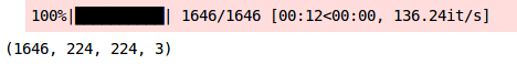
train_x = np.array(train_img)
    
    
 
    
    
train_x.shape
    
    
 
   
   

Create training and validation sets

  
  
   
   

    
    
# Define goals
    
    
 
    
    
train_y = train[‘emergency_or_not’].values
    
    
 
    
    
#Create validation set
    
    
 
    
    
train_x, val_x, train_y, val_y = train_test_split(train_x, train_y, test_size = 0.1, random_state = 13, stratify=train_y)
    
    
 
    
    
(train_x.shape, train_y.shape), (val_x.shape, val_y.shape)
    
    
 
   
   

Convert image to torch format

  
  
   
   

    
    
# Convert training images to torch format
    
    
 
    
    
train_x = train_x.reshape(1481, 3, 224, 224)
    
    
 
    
    
train_x  = torch.from_numpy(train_x)
    
    
 
    
    
# Convert target to torch format
    
    
 
    
    
train_y = train_y.astype(int)
    
    
 
    
    
train_y = torch.from_numpy(train_y)
    
    
 
    
    
# Convert verification image to torch format
    
    
 
    
    
val_x = val_x.reshape(165, 3, 224, 224)
    
    
 
    
    
val_x  = torch.from_numpy(val_x)
    
    
 
    
    
# Convert target to torch format
    
    
 
    
    
val_y = val_y.astype(int)
    
    
 
    
    
val_y = torch.from_numpy(val_y)
    
    
 
   
   

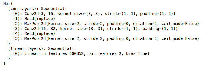
Define model architecture

  
  
   
   

    
    
torch.manual_seed(0)
    
    
 
    
    
class Net(Module):   
    
    
 
    
    
    def init ( self ): 
    
    
 
    
    
        super(Net, self).init()
    
    
 
    
    
        self.cnn_layers = Sequential(
    
    
 
    
    
            # Define 2D convolution layer
    
    
 
    
    
            Conv2d(3, 16, kernel_size=3, stride=1, padding=1),
    
    
 
    
    
            ReLU ( inplace = True ),
    
    
 
    
    
            MaxPool2d(kernel_size=2, stride=2),
    
    
 
    
    
            # Another 2D convolutional layer
    
    
 
    
    
            Conv2d(16, 32, kernel_size=3, stride=1, padding=1),
    
    
 
    
    
            ReLU ( inplace = True ),
    
    
 
    
    
            MaxPool2d(kernel_size=2, stride=2)
    
    
 
    
    
        )
    
    
 
    
    
        self.linear_layers = Sequential(
    
    
 
    
    
            Linear(32  56  56, 2)
    
    
 
    
    
        )
    
    
 
    
    
    # Propagation of the previous item
    
    
 
    
    
    def forward(self, x):
    
    
 
    
    
        x = self.cnn_layers(x)
    
    
 
    
    
        x = x.view(x.size(0), -1)
    
    
 
    
    
        x = self.linear_layers(x)
    
    
 
    
    
        return x
    
    
 
   
   

Define model parameters

  
  
   
   

    
    
# Define model
    
    
 
    
    
model = Net()
    
    
 
    
    
#Define optimizer
    
    
 
    
    
optimizer = Adam(model.parameters(), lr=0.0001)
    
    
 
    
    
# Define loss function
    
    
 
    
    
criterion = CrossEntropyLoss()
    
    
 
    
    
# Check if GPU is available
    
    
 
    
    
if torch.cuda.is_available():
    
    
 
    
    
    model = model.cuda()
    
    
 
    
    
    criterion = criterion.cuda()
    
    
 
    
    
print(model)
    
    
 
   
   

Training model

  
  
   
   

    
    
torch.manual_seed(0)
    
    
 
    
    
# Model batch size
    
    
 
    
    
batch_size = 128
    
    
 
    
    
# epoch number
    
    
 
    
    
n_epochs = 25
    
    
 
    
    
for epoch in range(1, n_epochs+1):
    
    
 
    
    
    # Keep records of training and validation set losses
    
    
 
    
    
    train_loss = 0.0
    
    
 
    
    
    permutation = torch.randperm(train_x.size()[0])
    
    
 
    
    
    training_loss = []
    
    
 
    
    
    for i in tqdm(range(0,train_x.size()[0], batch_size)):
    
    
 
    
    
        indices = permutation[i:i+batch_size]
    
    
 
    
    
        batch_x, batch_y = train_x[indices], train_y[indices]
    
    
 
    
    
        if torch.cuda.is_available():
    
    
 
    
    
            batch_x, batch_y = batch_x.cuda(), batch_y.cuda()
    
    
 
    
    
        optimizer.zero_grad()
    
    
 
    
    
        outputs = model(batch_x)
    
    
 
    
    
        loss = criterion(outputs,batch_y)
    
    
 
    
    
        training_loss.append(loss.item())
    
    
 
    
    
        loss.backward()
    
    
 
    
    
        optimizer.step()
    
    
 
    
    
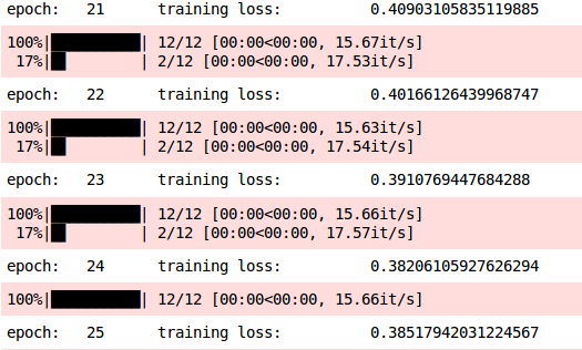
    training_loss = np.average(training_loss)
    
    
 
    
    
    print(‘epoch: \t’, epoch, ‘\t training loss: \t’, training_loss)
    
    
 
   
   

Prediction on training set

  
  
   
   

    
    
#Training set prediction
    
    
 
    
    
prediction = []
    
    
 
    
    
target = []
    
    
 
    
    
permutation = torch.randperm(train_x.size()[0])
    
    
 
    
    
for i in tqdm(range(0,train_x.size()[0], batch_size)):
    
    
 
    
    
    indices = permutation[i:i+batch_size]
    
    
 
    
    
    batch_x, batch_y = train_x[indices], train_y[indices]
    
    
 
    
    
    if torch.cuda.is_available():
    
    
 
    
    
        batch_x, batch_y = batch_x.cuda(), batch_y.cuda()
    
    
 
    
    
    with torch.no_grad():
    
    
 
    
    
        output = model(batch_x.cuda())
    
    
 
    
    
    softmax = torch.exp(output).cpu()
    
    
 
    
    
    prob = list(softmax.numpy())
    
    
 
    
    
    predictions = np.argmax(prob, axis=1)
    
    
 
    
    
    prediction.append(predictions)
    
    
 
    
    
    target.append(batch_y)
    
    
 
    
    
# Training set accuracy
    
    
 
    
    
accuracy = []
    
    
 
    
    
for i in range(len(prediction)):
    
    
 
    
    
    accuracy.append(accuracy_score(target[i],prediction[i]))
    
    
 
    
    
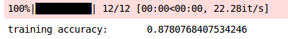
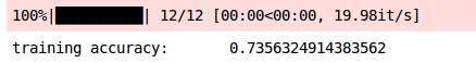
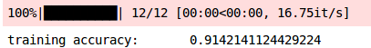
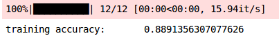
print(‘training accuracy: \t’, np.average(accuracy))
    
    
 
   
   

Prediction on validation set

  
  
   
   

    
    
# Validation set prediction
    
    
 
    
    
prediction_val = []
    
    
 
    
    
target_val = []
    
    
 
    
    
permutation = torch.randperm(val_x.size()[0])
    
    
 
    
    
for i in tqdm(range(0,val_x.size()[0], batch_size)):
    
    
 
    
    
    indices = permutation[i:i+batch_size]
    
    
 
    
    
    batch_x, batch_y = val_x[indices], val_y[indices]
    
    
 
    
    
    if torch.cuda.is_available():
    
    
 
    
    
        batch_x, batch_y = batch_x.cuda(), batch_y.cuda()
    
    
 
    
    
    with torch.no_grad():
    
    
 
    
    
        output = model(batch_x.cuda())
    
    
 
    
    
    softmax = torch.exp(output).cpu()
    
    
 
    
    
    prob = list(softmax.numpy())
    
    
 
    
    
    predictions = np.argmax(prob, axis=1)
    
    
 
    
    
    prediction_val.append(predictions)
    
    
 
    
    
    target_val.append(batch_y)
    
    
 
    
    
# Validation set accuracy
    
    
 
    
    
accuracy_val = []
    
    
 
    
    
for i in range(len(prediction_val)):
    
    
 
    
    
    accuracy_val.append(accuracy_score(target_val[i],prediction_val[i]))
    
    
 
    
    
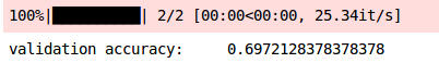
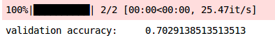
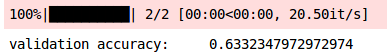
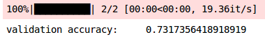
print(‘validation accuracy: \t’, np.average(accuracy_val))
    
    
 
   
   

This is our CNN model. The training accuracy is around 88%, and the verification accuracy is close to 70%.

We will work hard to improve the performance of this model. But before that, let's take a moment to understand the difficulties that may be responsible for this poor performance.

Deep learning problems

Deep Learning Dilemma 1: Lack of Available Data to Train Our Models

Deep learning models usually require large amounts of training data. Generally speaking, the more data, the better the model's performance. The problem with lack of data is that our deep learning model may not be able to learn patterns or features from the data, so it may not provide good performance on unseen data.

If you look at the car classification case study, we only have about 1650 images, so the model doesn't perform well on the validation set. The challenge of having little data is common when working with computer vision and deep learning models.

As you can imagine, collecting data manually is a tedious and time-consuming task. Therefore, instead of spending days collecting data, we can leverage data augmentation techniques .

Data augmentation is the process of generating new data or adding data to train a model without actually collecting the new data.

There are many data enhancement techniques for image data. Commonly used enhancement techniques include rotation, shearing, flipping, etc.

This is such a good topic that I decided to write a full article on it. My plan is to discuss these techniques and their implementation in PyTorch in the next article.

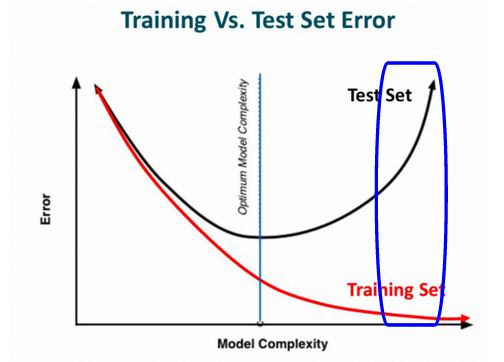
Deep Learning Conundrum #2: Model Overfitting

I'm sure you've heard of fitting. This is one of the most common dilemmas (and mistakes) data scientists make when new to machine learning. But this question actually transcends the field, and it applies to deep learning as well.

A model is considered overfitting when it performs very well on the training set, but performance degrades on the validation set (or unseen data).

For example, assume we have a training set and a validation set. We train the model using the training data and check its performance on the training and validation sets (the evaluation metric is accuracy). The training accuracy is 95% and the validation set accuracy is 62%. Sound familiar?

Since the validation accuracy is much lower than the training accuracy, it can be inferred that the model has an overfitting problem . The following example will give you a better understanding of what overfitting is:

The part marked in blue in the figure above is an overfitting model because the training error is very small and the test error is very high. The reason for overfitting is that the model learns unnecessary information even from the training data so that it performs very well on the training set.

However, when new data is introduced, it fails to perform. We can introduce Dropout into the model's architecture to solve the problem of overfitting .

Using Dropout, we randomly turn off certain neurons of the neural network. Suppose we add a dropout layer with probability 0.5 on top of the layer that originally had 20 neurons, so 10 of those 20 neurons will be suppressed and we end up with a less complex architecture.

Therefore, the model will not learn overly complex patterns and can avoid overfitting. Let us now add a Dropout layer to our architecture and check its performance.

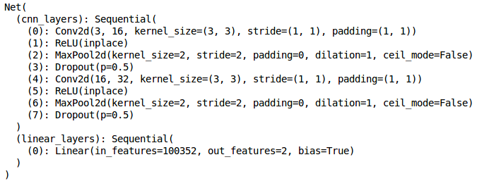
Model architecture

  
  
   
   

    
    
torch.manual_seed(0)
    
    
 
    
    
class Net(Module):   
    
    
 
    
    
    def init ( self ): 
    
    
 
    
    
        super(Net, self).init()
    
    
 
    
    
        self.cnn_layers = Sequential(
    
    
 
    
    
            # Define 2D convolution layer
    
    
 
    
    
            Conv2d(3, 16, kernel_size=3, stride=1, padding=1),
    
    
 
    
    
            ReLU ( inplace = True ),
    
    
 
    
    
            MaxPool2d(kernel_size=2, stride=2),
    
    
 
    
    
            # Dropout layer
    
    
 
    
    
            Dropout(),
    
    
 
    
    
            #Another 2D convolutional layer
    
    
 
    
    
            Conv2d(16, 32, kernel_size=3, stride=1, padding=1),
    
    
 
    
    
            ReLU ( inplace = True ),
    
    
 
    
    
            MaxPool2d(kernel_size=2, stride=2),
    
    
 
    
    
            # Dropout layer
    
    
 
    
    
            Dropout(),
    
    
 
    
    
        )
    
    
 
    
    
        self.linear_layers = Sequential(
    
    
 
    
    
            Linear(32  56  56, 2)
    
    
 
    
    
        )
    
    
 
    
    
    # forward propagation  
    
    
 
    
    
    def forward(self, x):
    
    
 
    
    
        x = self.cnn_layers(x)
    
    
 
    
    
        x = x.view(x.size(0), -1)
    
    
 
    
    
        x = self.linear_layers(x)
    
    
 
    
    
        return x
    
    
 
   
   

Here, I added a dropout layer to each convolution block. The default value is 0.5, which means half of the neurons will be randomly turned off. This is a hyperparameter and you can choose any value between 0 and 1.

Next, we will define the parameters of the model, such as the loss function, optimizer, and learning rate.

Model parameters

  
  
   
   

    
    
# Define model
    
    
 
    
    
model = Net()
    
    
 
    
    
#Define optimizer
    
    
 
    
    
optimizer = Adam(model.parameters(), lr=0.0001)
    
    
 
    
    
# Define loss function
    
    
 
    
    
criterion = CrossEntropyLoss()
    
    
 
    
    
# Check if GPU is available
    
    
 
    
    
if torch.cuda.is_available():
    
    
 
    
    
    model = model.cuda()
    
    
 
    
    
    criterion = criterion.cuda()
    
    
 
    
    
print(model)
    
    
 
   
   

Here you can see that the default value in Dropout is 0.5. Finally, let's train the model after adding the Dropout layer:

Training model

  
  
   
   

    
    
torch.manual_seed(0)
    
    
 
    
    
# Model batch size
    
    
 
    
    
batch_size = 128
    
    
 
    
    
# epoch number
    
    
 
    
    
n_epochs = 25
    
    
 
    
    
for epoch in range(1, n_epochs+1):
    
    
 
    
    
    # Keep records of training and validation set losses
    
    
 
    
    
    train_loss = 0.0
    
    
 
    
    
    permutation = torch.randperm(train_x.size()[0])
    
    
 
    
    
    training_loss = []
    
    
 
    
    
    for i in tqdm(range(0,train_x.size()[0], batch_size)):
    
    
 
    
    
        indices = permutation[i:i+batch_size]
    
    
 
    
    
        batch_x, batch_y = train_x[indices], train_y[indices]
    
    
 
    
    
        if torch.cuda.is_available():
    
    
 
    
    
            batch_x, batch_y = batch_x.cuda(), batch_y.cuda()
    
    
 
    
    
        optimizer.zero_grad()
    
    
 
    
    
        outputs = model(batch_x)
    
    
 
    
    
        loss = criterion(outputs,batch_y)
    
    
 
    
    
        training_loss.append(loss.item())
    
    
 
    
    
        loss.backward()
    
    
 
    
    
        optimizer.step()
    
    
 
    
    
    training_loss = np.average(training_loss)
    
    
 
    
    
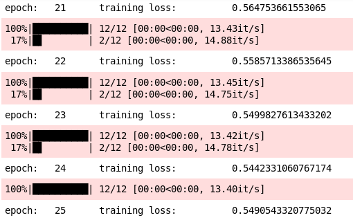
    print(‘epoch: \t’, epoch, ‘\t training loss: \t’, training_loss)
    
    
 
   
   

Now, let us check the training and validation accuracy using this trained model.

Check model performance

  
  
   
   

    
    
# 
    
    
 
    
    
prediction = []
    
    
 
    
    
target = []
    
    
 
    
    
permutation = torch.randperm(train_x.size()[0])
    
    
 
    
    
for i in tqdm(range(0,train_x.size()[0], batch_size)):
    
    
 
    
    
    indices = permutation[i:i+batch_size]
    
    
 
    
    
    batch_x, batch_y = train_x[indices], train_y[indices]
    
    
 
    
    
    if torch.cuda.is_available():
    
    
 
    
    
        batch_x, batch_y = batch_x.cuda(), batch_y.cuda()
    
    
 
    
    
    with torch.no_grad():
    
    
 
    
    
        output = model(batch_x.cuda())
    
    
 
    
    
    softmax = torch.exp(output).cpu()
    
    
 
    
    
    prob = list(softmax.numpy())
    
    
 
    
    
    predictions = np.argmax(prob, axis=1)
    
    
 
    
    
    prediction.append(predictions)
    
    
 
    
    
    target.append(batch_y)
    
    
 
    
    
# Training set accuracy
    
    
 
    
    
accuracy = []
    
    
 
    
    
for i in range(len(prediction)):
    
    
 
    
    
    accuracy.append(accuracy_score(target[i],prediction[i]))
    
    
 
    
    
print(‘training accuracy: \t’, np.average(accuracy))
    
    
 
   
   

Again, let's check the validation set accuracy:

  
  
   
   

    
    
# Validation set prediction
    
    
 
    
    
prediction_val = []
    
    
 
    
    
target_val = []
    
    
 
    
    
permutation = torch.randperm(val_x.size()[0])
    
    
 
    
    
for i in tqdm(range(0,val_x.size()[0], batch_size)):
    
    
 
    
    
    indices = permutation[i:i+batch_size]
    
    
 
    
    
    batch_x, batch_y = val_x[indices], val_y[indices]
    
    
 
    
    
    if torch.cuda.is_available():
    
    
 
    
    
        batch_x, batch_y = batch_x.cuda(), batch_y.cuda()
    
    
 
    
    
    with torch.no_grad():
    
    
 
    
    
        output = model(batch_x.cuda())
    
    
 
    
    
    softmax = torch.exp(output).cpu()
    
    
 
    
    
    prob = list(softmax.numpy())
    
    
 
    
    
    predictions = np.argmax(prob, axis=1)
    
    
 
    
    
    prediction_val.append(predictions)
    
    
 
    
    
    target_val.append(batch_y)
    
    
 
    
    
# Validation set accuracy
    
    
 
    
    
accuracy_val = []
    
    
 
    
    
for i in range(len(prediction_val)):
    
    
 
    
    
    accuracy_val.append(accuracy_score(target_val[i],prediction_val[i]))
    
    
 
    
    
print(‘validation accuracy: \t’, np.average(accuracy_val))
    
    
 
   
   

Let's compare this with previous results:

	Training set accuracy	Validation set accuracy
No Dropout	87.80	69.72
There is Dropout	73.56	70.29

The above table represents the accuracy without Dropout and with Dropout. If you look at the training and validation accuracy of models without omissions, they are out of sync. The training accuracy is too high and the verification accuracy is low. Therefore, this may be an example of overfitting.

When we introduce Dropout, the accuracy of the training and validation sets is synchronized. Therefore, if your model is overfitting, you can try adding a Dropout layer to reduce the complexity of the model .

The number of Dropouts to add is a hyperparameter that you can manipulate with. Now let's look at another puzzle.

Deep learning problem 3: Model underfitting

It is also possible for deep learning models to underfit, which may sound unlikely.

Underfitting is when the model is unable to learn patterns from the training data itself, and therefore performs lower on the training set.

This may be due to a variety of reasons, such as not having enough data to train, the architecture being too simple, the model being trained less often, etc.

To overcome the underfitting problem, you can try the following solutions:

1. Add training data
2. Make a complex model
3. Increase training epochs

For our problem, underfitting is not an issue, so we will move on to the next method of improving the performance of deep learning models.

Deep learning problem 4: Training takes too long

In some cases, you may find that your neural network takes a lot of time to converge. The main reason behind this is the change in the distribution of inputs to the neural network layers.

During the training process, the weights of each layer of the neural network change, and the activations also change accordingly. Now, these activations are the input to the next layer, so each successive iteration changes the distribution.

Because of this distribution change, each layer must adapt to changing inputs—which is why training times increase.

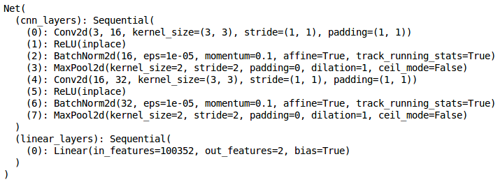
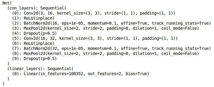
To overcome this problem, we can apply batch normalization, where we normalize the activations of the hidden layers and try to make the same distribution.

Let us now add a batchnorm layer to the architecture and check its performance on the vehicle classification problem:

  
  
   
   

    
    
torch.manual_seed(0)
    
    
 
    
    
class Net(Module):   
    
    
 
    
    
    def init ( self ): 
    
    
 
    
    
        super(Net, self).init()
    
    
 
    
    
        self.cnn_layers = Sequential(
    
    
 
    
    
            # Define 2D convolution layer
    
    
 
    
    
            Conv2d(3, 16, kernel_size=3, stride=1, padding=1),
    
    
 
    
    
            ReLU ( inplace = True ),
    
    
 
    
    
            # BN layer
    
    
 
    
    
            BatchNorm2d ( 16 ),
    
    
 
    
    
            MaxPool2d(kernel_size=2, stride=2),
    
    
 
    
    
            #Another 2D convolutional layer
    
    
 
    
    
            Conv2d(16, 32, kernel_size=3, stride=1, padding=1),
    
    
 
    
    
            ReLU ( inplace = True ),    
    
    
 
    
    
            # BN layer
    
    
 
    
    
            BatchNorm2d ( 32 ),
    
    
 
    
    
            MaxPool2d(kernel_size=2, stride=2),
    
    
 
    
    
        )
    
    
 
    
    
        self.linear_layers = Sequential(
    
    
 
    
    
            Linear(32  56  56, 2)
    
    
 
    
    
        )
    
    
 
    
    
    # forward propagation  
    
    
 
    
    
    def forward(self, x):
    
    
 
    
    
        x = self.cnn_layers(x)
    
    
 
    
    
        x = x.view(x.size(0), -1)
    
    
 
    
    
        x = self.linear_layers(x)
    
    
 
    
    
        return x
    
    
 
   
   

Define model parameters

  
  
   
   

    
    
# Define model
    
    
 
    
    
model = Net()
    
    
 
    
    
#Define optimizer
    
    
 
    
    
optimizer = Adam(model.parameters(), lr=0.00005)
    
    
 
    
    
# Define loss function
    
    
 
    
    
criterion = CrossEntropyLoss()
    
    
 
    
    
# Check if GPU is available
    
    
 
    
    
if torch.cuda.is_available():
    
    
 
    
    
    model = model.cuda()
    
    
 
    
    
    criterion = criterion.cuda()
    
    
 
    
    
print(model)
    
    
 
   
   

Let's train the model

  
  
   
   

    
    
torch.manual_seed(0)
    
    
 
    
    
# Model batch size
    
    
 
    
    
batch_size = 128
    
    
 
    
    
# epoch number
    
    
 
    
    
n_epochs = 5
    
    
 
    
    
for epoch in range(1, n_epochs+1):
    
    
 
    
    
    # Keep records of training and validation set losses
    
    
 
    
    
    train_loss = 0.0
    
    
 
    
    
    permutation = torch.randperm(train_x.size()[0])
    
    
 
    
    
    training_loss = []
    
    
 
    
    
    for i in tqdm(range(0,train_x.size()[0], batch_size)):
    
    
 
    
    
        indices = permutation[i:i+batch_size]
    
    
 
    
    
        batch_x, batch_y = train_x[indices], train_y[indices]
    
    
 
    
    
        if torch.cuda.is_available():
    
    
 
    
    
            batch_x, batch_y = batch_x.cuda(), batch_y.cuda()
    
    
 
    
    
        optimizer.zero_grad()
    
    
 
    
    
        outputs = model(batch_x)
    
    
 
    
    
        loss = criterion(outputs,batch_y)
    
    
 
    
    
        training_loss.append(loss.item())
    
    
 
    
    
        loss.backward()
    
    
 
    
    
        optimizer.step()
    
    
 
    
    
    training_loss = np.average(training_loss)
    
    
 
    
    
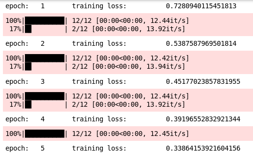
    print(‘epoch: \t’, epoch, ‘\t training loss: \t’, training_loss)
    
    
 
   
   

Clearly, the model is able to learn very quickly. At the 5th epoch, our training loss is 0.3386, and it takes 25 epochs before our training loss is 0.3851 when we do not use batch normalization.

Therefore, the introduction of batch normalization undoubtedly reduces the training time. Let's check the performance on training and validation sets:

  
  
   
   

    
    
prediction = []
    
    
 
    
    
target = []
    
    
 
    
    
permutation = torch.randperm(train_x.size()[0])
    
    
 
    
    
for i in tqdm(range(0,train_x.size()[0], batch_size)):
    
    
 
    
    
    indices = permutation[i:i+batch_size]
    
    
 
    
    
    batch_x, batch_y = train_x[indices], train_y[indices]
    
    
 
    
    
    if torch.cuda.is_available():
    
    
 
    
    
        batch_x, batch_y = batch_x.cuda(), batch_y.cuda()
    
    
 
    
    
    with torch.no_grad():
    
    
 
    
    
        output = model(batch_x.cuda())
    
    
 
    
    
    softmax = torch.exp(output).cpu()
    
    
 
    
    
    prob = list(softmax.numpy())
    
    
 
    
    
    predictions = np.argmax(prob, axis=1)
    
    
 
    
    
    prediction.append(predictions)
    
    
 
    
    
    target.append(batch_y)
    
    
 
    
    
# Training set accuracy
    
    
 
    
    
accuracy = []
    
    
 
    
    
for i in range(len(prediction)):
    
    
 
    
    
    accuracy.append(accuracy_score(target[i],prediction[i]))
    
    
 
    
    
print(‘training accuracy: \t’, np.average(accuracy))
    
    
 
   
   

  
  
   
   

    
    
# Validation set prediction
    
    
 
    
    
prediction_val = []
    
    
 
    
    
target_val = []
    
    
 
    
    
permutation = torch.randperm(val_x.size()[0])
    
    
 
    
    
for i in tqdm(range(0,val_x.size()[0], batch_size)):
    
    
 
    
    
    indices = permutation[i:i+batch_size]
    
    
 
    
    
    batch_x, batch_y = val_x[indices], val_y[indices]
    
    
 
    
    
    if torch.cuda.is_available():
    
    
 
    
    
        batch_x, batch_y = batch_x.cuda(), batch_y.cuda()
    
    
 
    
    
    with torch.no_grad():
    
    
 
    
    
        output = model(batch_x.cuda())
    
    
 
    
    
    softmax = torch.exp(output).cpu()
    
    
 
    
    
    prob = list(softmax.numpy())
    
    
 
    
    
    predictions = np.argmax(prob, axis=1)
    
    
 
    
    
    prediction_val.append(predictions)
    
    
 
    
    
    target_val.append(batch_y)
    
    
 
    
    
# Validation set accuracy
    
    
 
    
    
accuracy_val = []
    
    
 
    
    
for i in range(len(prediction_val)):
    
    
 
    
    
    accuracy_val.append(accuracy_score(target_val[i],prediction_val[i]))
    
    
 
    
    
print(‘validation accuracy: \t’, np.average(accuracy_val))
    
    
 
   
   

Adding batch normalization can reduce training time, but there is a problem. Can you figure out what it is? The model is now overfitted as we have an accuracy of 91% on the training set and 63% on the validation set. Remember, we did not add a Dropout layer to the latest model.

These are some techniques we can use to improve the performance of deep learning models. Now, let's combine all the techniques we've learned so far.

Case Study: Improving the Performance of Vehicle Classification Models

We have seen how dropout and batch normalization help reduce overfitting and speed up the training process. Now it's time to bring all these technologies together and build a model.

  
  
   
   

    
    
torch.manual_seed(0)
    
    
 
    
    
class Net(Module):   
    
    
 
    
    
    def init ( self ): 
    
    
 
    
    
        super(Net, self).init()
    
    
 
    
    
        self.cnn_layers = Sequential(
    
    
 
    
    
            # Define 2D convolution layer
    
    
 
    
    
            Conv2d(3, 16, kernel_size=3, stride=1, padding=1),
    
    
 
    
    
            ReLU ( inplace = True ),
    
    
 
    
    
            # BN layer
    
    
 
    
    
            BatchNorm2d ( 16 ),
    
    
 
    
    
            MaxPool2d(kernel_size=2, stride=2),
    
    
 
    
    
            # Add dropout
    
    
 
    
    
            Dropout(),
    
    
 
    
    
            #Another 2D convolutional layer
    
    
 
    
    
            Conv2d(16, 32, kernel_size=3, stride=1, padding=1),
    
    
 
    
    
            ReLU ( inplace = True ),
    
    
 
    
    
            # BN layer
    
    
 
    
    
            BatchNorm2d ( 32 ),
    
    
 
    
    
            MaxPool2d(kernel_size=2, stride=2),
    
    
 
    
    
            # Add dropout
    
    
 
    
    
            Dropout(),
    
    
 
    
    
        )
    
    
 
    
    
        self.linear_layers = Sequential(
    
    
 
    
    
            Linear(32  56  56, 2)
    
    
 
    
    
        )
    
    
 
    
    
    # forward propagation  
    
    
 
    
    
    def forward(self, x):
    
    
 
    
    
        x = self.cnn_layers(x)
    
    
 
    
    
        x = x.view(x.size(0), -1)
    
    
 
    
    
        x = self.linear_layers(x)
    
    
 
    
    
        return x
    
    
 
   
   

Now, we will define the parameters of the model:

  
  
   
   

    
    
# Define model
    
    
 
    
    
model = Net()
    
    
 
    
    
#Define optimizer
    
    
 
    
    
optimizer = Adam(model.parameters(), lr=0.00025)
    
    
 
    
    
# Define loss function
    
    
 
    
    
criterion = CrossEntropyLoss()
    
    
 
    
    
# Check if GPU is available
    
    
 
    
    
if torch.cuda.is_available():
    
    
 
    
    
    model = model.cuda()
    
    
 
    
    
    criterion = criterion.cuda()
    
    
 
    
    
print(model)
    
    
 
   
   

Finally, let's train the model:

  
  
   
   

    
    
torch.manual_seed(0)
    
    
 
    
    
# Model batch size
    
    
 
    
    
batch_size = 128
    
    
 
    
    
# epoch number
    
    
 
    
    
n_epochs = 10
    
    
 
    
    
for epoch in range(1, n_epochs+1):
    
    
 
    
    
    # Keep records of training and validation set losses
    
    
 
    
    
    train_loss = 0.0
    
    
 
    
    
    permutation = torch.randperm(train_x.size()[0])
    
    
 
    
    
    training_loss = []
    
    
 
    
    
    for i in tqdm(range(0,train_x.size()[0], batch_size)):
    
    
 
    
    
        indices = permutation[i:i+batch_size]
    
    
 
    
    
        batch_x, batch_y = train_x[indices], train_y[indices]
    
    
 
    
    
        if torch.cuda.is_available():
    
    
 
    
    
            batch_x, batch_y = batch_x.cuda(), batch_y.cuda()
    
    
 
    
    
        optimizer.zero_grad()
    
    
 
    
    
        outputs = model(batch_x)
    
    
 
    
    
        loss = criterion(outputs,batch_y)
    
    
 
    
    
        training_loss.append(loss.item())
    
    
 
    
    
        loss.backward()
    
    
 
    
    
        optimizer.step()
    
    
 
    
    
    training_loss = np.average(training_loss)
    
    
 
    
    
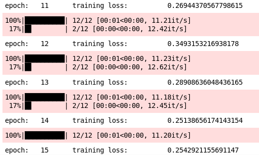
    print(‘epoch: \t’, epoch, ‘\t training loss: \t’, training_loss)
    
    
 
   
   

Next, let's check the model's performance:

  
  
   
   

    
    
prediction = []
    
    
 
    
    
target = []
    
    
 
    
    
permutation = torch.randperm(train_x.size()[0])
    
    
 
    
    
for i in tqdm(range(0,train_x.size()[0], batch_size)):
    
    
 
    
    
    indices = permutation[i:i+batch_size]
    
    
 
    
    
    batch_x, batch_y = train_x[indices], train_y[indices]
    
    
 
    
    
    if torch.cuda.is_available():
    
    
 
    
    
        batch_x, batch_y = batch_x.cuda(), batch_y.cuda()
    
    
 
    
    
    with torch.no_grad():
    
    
 
    
    
        output = model(batch_x.cuda())
    
    
 
    
    
    softmax = torch.exp(output).cpu()
    
    
 
    
    
    prob = list(softmax.numpy())
    
    
 
    
    
    predictions = np.argmax(prob, axis=1)
    
    
 
    
    
    prediction.append(predictions)
    
    
 
    
    
    target.append(batch_y)
    
    
 
    
    
# Training set accuracy
    
    
 
    
    
accuracy = []
    
    
 
    
    
for i in range(len(prediction)):
    
    
 
    
    
    accuracy.append(accuracy_score(target[i],prediction[i]))
    
    
 
    
    
print(‘training accuracy: \t’, np.average(accuracy))
    
    
 
   
   

  
  
   
   

    
    
# Validation set prediction
    
    
 
    
    
prediction_val = []
    
    
 
    
    
target_val = []
    
    
 
    
    
permutation = torch.randperm(val_x.size()[0])
    
    
 
    
    
for i in tqdm(range(0,val_x.size()[0], batch_size)):
    
    
 
    
    
    indices = permutation[i:i+batch_size]
    
    
 
    
    
    batch_x, batch_y = val_x[indices], val_y[indices]
    
    
 
    
    
    if torch.cuda.is_available():
    
    
 
    
    
        batch_x, batch_y = batch_x.cuda(), batch_y.cuda()
    
    
 
    
    
    with torch.no_grad():
    
    
 
    
    
        output = model(batch_x.cuda())
    
    
 
    
    
    softmax = torch.exp(output).cpu()
    
    
 
    
    
    prob = list(softmax.numpy())
    
    
 
    
    
    predictions = np.argmax(prob, axis=1)
    
    
 
    
    
    prediction_val.append(predictions)
    
    
 
    
    
    target_val.append(batch_y)
    
    
 
    
    
# Validation set accuracy
    
    
 
    
    
accuracy_val = []
    
    
 
    
    
for i in range(len(prediction_val)):
    
    
 
    
    
    accuracy_val.append(accuracy_score(target_val[i],prediction_val[i]))
    
    
 
    
    
print(‘validation accuracy: \t’, np.average(accuracy_val))
    
    
 
   
   

The verification accuracy is significantly improved to 73%. marvelous!

end

In this article, we examine the different challenges you may face when using deep learning models such as CNNs. We also learned the solutions to all these puzzles, and finally, we built a model using these solutions.

After we added these techniques to the model, the model's accuracy improved on the validation set. There is always room for improvement, and here are some things you can try:

• Adjust Dropout rate
• Increase or decrease the number of convolutional layers
• Increase or decrease the number of Dense layers
• Adjust the number of neurons in the hidden layer, etc.