Generalization of deep learning models

This content cannot be displayed outside Feishu documents at the moment.

Zero, generalizability

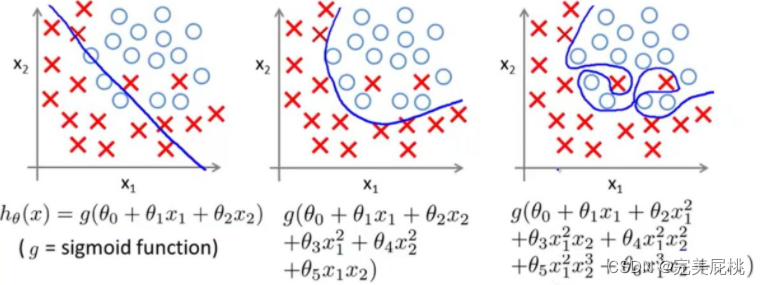
Generalizability refers to the ability of a model to be applied to new data and make accurate predictions after training. A model is often trained too well on the training data, that is, overfitted, and fails to generalize.

The reasons for overfitting of deep learning models are not only due to data reasons :

Model complexity is too high : If the model has too many parameters or layers, it can easily remember the details of the training data but cannot generalize to new data. This can cause the model to perform poorly on test data.
Insufficient training data : If the amount of training data is too small, the model may not be able to capture the true distribution of the data and is therefore prone to overfitting. More training data usually helps improve the generalization performance of the model.
Improper feature selection : Selecting features that are irrelevant to the problem or redundant may lead to overfitting. Good feature selection is crucial for model performance.
Training takes too long : If the training takes too long, the model may remember noise instead of the true data patterns. Using techniques like early stopping during training can help avoid this.
Lack of regularization : Regularization techniques such as L1 regularization and L2 regularization can limit the size of model parameters, prevent the model from being too complex, and help alleviate overfitting.
Data imbalance : If the number of samples between different classes in the training data is very different, the model may tend to predict the class with more samples and ignore other classes.
Noisy data : Noise or mislabeling in the training data can cause the model to overfit as the model tries to adapt to this noise.
Missing features : If features that are not present in the training data appear in the test data, the model may not be able to handle these situations, resulting in performance degradation.
Randomness : Deep learning models usually have a certain degree of randomness, which can lead to unstable training results if the model is initialized or the data is not partitioned properly.

How to solve overfitting? Improve generalization?

1. Regular technology

1. Display regularity

(1) Dropout: A Simple Way to Prevent Neural Networks from Overfitting (starting from the network)

Dropout is applied between adjacent layers in the network. The key idea is to randomly select some neurons and set their output to zero in each training iteration. These neurons do not participate in forward and backpropagation in this iteration. The key to Dropout is to drop neurons with a certain probability (usually 0.5). This probability is called the dropout rate. During the test phase, all neurons participate in forward propagation, but their outputs are scaled by the dropout rate to maintain the desired output value.

Why Dropout can prevent overfitting?

Dropout helps reduce the co-adaptation between neurons in the neural network and reduces the model's over-reliance on certain specific features, thereby improving generalization performance . Because of the dropout procedure, two neurons do not necessarily appear in a dropout network every time. In this way, the update of weights no longer relies on the joint action of hidden nodes with fixed relationships, preventing certain features from being effective only under other specific features. This forces the network to learn more robust features that are also present in random subsets of other neurons. In other words, if our neural network is making some kind of prediction, it should not be too sensitive to some specific clue fragments. Even if specific clues are lost, it should be able to learn some common features from many other clues. From this perspective, dropout is a bit like L1 and L2 regularization. Reducing weights makes the network more robust to the loss of specific neuron connections.
By randomly discarding neurons, Dropout is equivalent to training multiple different sub-models , which jointly learn to solve problems, thus improving the robustness of the model.

(2) Data augmentation (starting from samples)

Data augmentation is a powerful technique used to improve the generalization performance of deep learning models. Data augmentation generates new training samples by performing a series of random transformations and expansions on the training data, thereby increasing the diversity of model learning and mitigating the overfitting problem.
Why does data augmentation prevent overfitting?

A popular way to understand overfitting is: too many parameters and too few samples. Data augmentation is equivalent to adding samples, so that although the semantic information conveyed is the same, they are different in the eyes of the model. The goal is that the model never views the exact same image twice while training. This allows the model to observe more of the data and thus have better generalization capabilities. The general approach is as follows:

1) Collect more data from data sources

2) Copy the original data and add random noise

3) Resampling

4) Estimate data distribution parameters based on the current data set, use this distribution to generate more data, etc.

(3)NoiseNoise

A common type of regularization is to inject noise during training: noise is added to or multiplied by the hidden units of the neural network. By allowing some inaccuracies when training deep neural networks, you not only improve training performance but also improve model accuracy. In addition to adding noise to the input data itself, noise can be added to activations, weights, or gradients. Too little noise has no effect, while too much noise makes learning the mapping function too difficult.

2. Implicit regularity

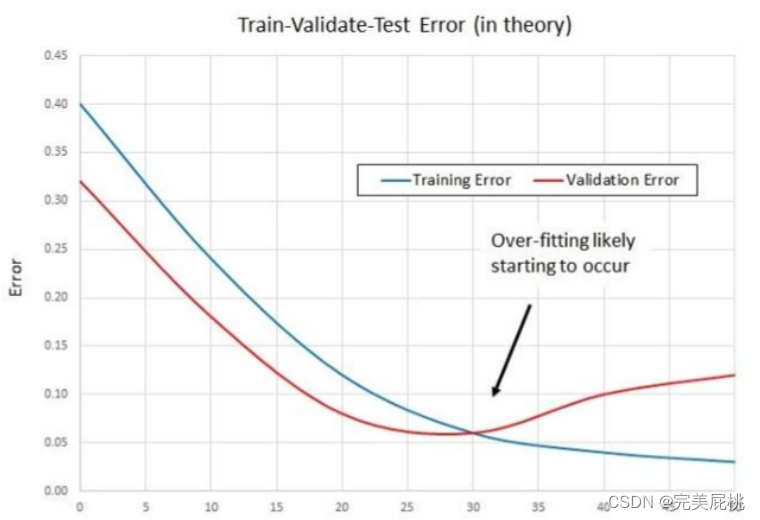
(1) Early Stop

Early stopping is a method of truncating the number of iterations to prevent overfitting, that is, stopping iteration before the model iteratively converges on the training data set to prevent overfitting . This is a cross-validation strategy where we retain a portion of the training set as the validation set. When we see performance getting worse on the validation set, we stop training the model. Because when initializing the network, the weights are usually initially smaller. The longer the training time, the larger the weights of some networks may be. If we stop training at the right time, we can limit the capabilities of the network to a certain range.

(2)Batch Normalization

Batch Normalization (BN, Batch Normalization) is a technique that normalizes the network input, applied to the activation of the previous layer or the direct input. This method allows each layer of the network to learn as independently as possible from other layers. BN normalizes the input layer by adjusting and scaling activations.

This is a very useful regularization method that can speed up the training of large convolutional networks many times, and at the same time, the accuracy of classification after convergence can also be greatly improved. When BN trains a certain layer, it will normalize each mini-batch data to normalize the output to the normal distribution of N(0,1), reducing the Internal convariate shift (change in internal neuron distribution) , When training traditional deep neural networks, the distribution of inputs in each layer is changing, so training is difficult. You can only choose to use a very small learning rate. However, after using BN in each layer, this can be effectively solved. Problem, the learning rate can be increased many times.

2. Model optimization

Feature engineering :
1. Designing and selecting appropriate features can help the model better capture patterns in the data and improve generalization performance.
Model selection :
1. Choose an appropriate model architecture and model type based on the nature of the problem and available data to improve generalization performance.

Understanding Deep Learning (Still) Requires Rethinking Generalization（ACM2021)

The article stated:

(1) Training process and overfitting : Deep learning models usually have a large number of parameters, which allows the model to perform very well on the training data, but it is also easy to overmemorize (overfit) the noise and details of the training data. Overfitting is when a model performs poorly on unseen data.

(2) The relationship between overfitting and generalization : The relationship between overfitting and generalization is an important issue in deep learning. The article points out that although we know that overfitting is a problem on training data, the relationship between the degree of overfitting and the generalization performance of the model on unseen data is not straightforward. This is because the model may generalize by learning the structure of a low-dimensional manifold in a high-dimensional space, rather than simply memorizing the training data.

(3) Optimization methods and implicit regularization effects : The article puts forward an interesting point, that is, optimization methods such as stochastic gradient descent (SGD) themselves may have implicit regularization effects. SGD is a stochastic method that uses random mini-batches of data to update model parameters in each training iteration. The author believes that this randomness of SGD can limit the solution space of the model, making the learned model have a certain generalization ability. This means that the optimization method itself plays a certain role in reducing the risk of overfitting and improving generalization performance.

3. Counterattack

Adding adversarial data to the machine learning model can obtain deceptive identification results. If we can enhance the model's attack resistance, we can naturally improve the model's generalization ability.

Paper address: Adversarial Training Towards Robust Multimedia Recommender System (IEEE'2020)

Code: https://github.com/duxy-me/AMR

Motivation: The author proposes that the existing visual multi-modal recommendation model is not robust enough. After adding a small artificial noise perturbation (adversarial sample) to the input image, the ranking of the recommendation list may change significantly, as shown in the figure below.

Innovation: The author draws on ideas from the field of visual security and proposes an adversarial training method to obtain a more robust and efficient recommendation model. Adversarial training can simply be considered a special data enhancement method.

Method: The training process of the AMR model can be understood as a minimaxprocess of playing a game. The disturbance noise is obtained by maximizing the loss function of VBPR, and the parameters of the model are obtained by minimizing the VBPR loss function and the adversarial loss function. Similar to the idea of the GAN model, this method forces the model to become more robust.

The training process is similar to a minimax game : The article mentioned that the training of the AMR model can be regarded as a minimax game, in which the two main players are the model itself and a kind of disturbance noise. This means that the training process involves two competing objectives or loss functions.
VBPR loss function : VBPR is a model for multimedia recommendation that combines the user's historical behavioral data and the visual information of the product to predict the products the user may like and perform personalized ranking. During training, the loss function of VBPR is used to minimize the prediction error of the model to make it perform better in personalized recommendations.
Adversarial loss function : During training, an adversarial loss function is introduced. This means that there is an adversarial attacker (perturbation noise) whose goal is to maximize the VBPR loss function. That is, the attacker attempts to degrade the performance of the VBPR model by adding noise to the input data, thereby increasing the misleading of recommendations.
Optimization of model parameters : During the training process, the parameters of the model will be affected by two loss functions at the same time. On the one hand, the model will try to reduce the VBPR loss function to improve the performance of personalized recommendations. On the other hand, the model needs to be resistant to the noise of adversarial attackers, so the adversarial loss function needs to be minimized to maintain the stability of its performance.
Adversarial training and robustness : This training process is similar to the ideas in generative adversarial networks (GANs), where generators and discriminators compete with each other to generate more realistic data. Here, the purpose of adversarial training is to enhance the robustness of the recommendation system so that it can resist external attacks and interference while providing more accurate personalized recommendations.

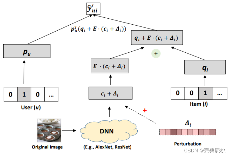
yˆuiIt is the predicted value of the user 's rating ufor the product .i
puis the user u's latent vector (or feature vector), used to represent the user's characteristics.
qiis ithe latent vector (or feature vector) of the product, which is used to represent the characteristics of the product.
Eis an error matrix that represents additional noise or errors, usually assumed to obey some probability distribution.
ciis ia vector of contextual information of the product, used to represent the environmental or contextual features of the product.
∆iis ian additional offset for commodity , which can be understood as ia correction term for commodity .

The goal of this formula is to predict the user's rating of the item through the feature vectors of the user and the item, as well as additional contextual information and errors. Typically, the model training process adjusts the latent vectors puand qito minimize the error between the true and predicted ratings. Error terms Eand contextual information cican be used to capture noise and environmental information in the model to improve prediction accuracy.

Since the image feature extraction model is usually trained separately from the recommendation model, the author proposes to directly add adversarial perturbations to the extracted image representation (embedding). User u's preference for item i is as follows, which is the user's preference for item without adding noise.

Δi represents the perturbation noise added to the image embedding, and ε is a hyperparameter that controls the magnitude of the perturbation.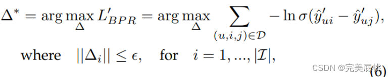

The parameters of the model are obtained by optimizing the following loss function:

y_ui is the user's preference for items without disturbing noise, and λ is a hyperparameter that controls the intensity of adversarial training. When λ=0, AMP is degraded to VBPR, and adversarial loss can be regarded as a special regularization term.

4. Transfer learning

1. Domain usually refers to the distribution and feature space of data. Domain includes the following elements:

Data Distribution : Domain relates to the distribution of training and test data. In transfer learning, there is usually a source domain and a target domain. The source domain is the domain that the model is initially trained on, while the target domain is the domain that the model ultimately needs to perform well on. The data distribution of these two domains may be different, that is, there are differences in their characteristics, statistical properties, etc.

Source Domain : This is the domain that the model comes into contact with during the training process. It is usually labeled data used for model training.
Target Domain : This is the domain to which the model is adapted when testing or applying, usually with no or very few labeled data.

Task : Domains are also often related to tasks. There are usually one or more related tasks in the source domain, and the goal of transfer learning is to transfer the knowledge of these tasks to new tasks in the target domain. This means that the tasks of the source domain and the target domain may be different, but there may be some degree of correlation between them.

2. Domain Adaptation :

Domain adaptation is a transfer learning problem in which a model is trained on a source domain and attempts to transfer its knowledge to one or more related tasks on a target domain.
The source domain and the target domain usually have some correlation , but there may be some differences in their data distribution. The goal of domain adaptation is to improve the performance of the model in the target domain by reducing the distribution difference between the source domain and the target domain.
Domain adaptation assumes that tasks between source and target domains are relevant , so it aims to enable the model to adapt to the data distribution of the target domain to improve the performance of tasks on the target domain.

3. Domain Generalization :

Domain generalization is a more challenging transfer learning problem, where a model is trained on multiple source domains and then attempts to generalize on an unseen target domain, regardless of the specific task on the target domain.
Domain generalization assumes that the tasks between the source domain and the target domain are irrelevant , and its goal is to achieve good generalization performance in the target domain independent of the tasks in the source domain.
Domain generalization aims to make the model generalize better even if there is no task-specific label information on the target domain.

4. Bias refers to errors introduced by using simplified models to approximate real-world problems. It represents the difference between the average predicted value of the model and the true value. High bias indicates that the model does not fit the data well enough to capture underlying patterns and relationships.

5. Variance refers to the variability of model predictions across different training sets. It measures the sensitivity of the model to fluctuations in the training data. High variance indicates that the model is overfitting the data and is too sensitive to noise and random changes.

6. Pseudo-labeling attempts to assign labels to unlabeled data by using labeled data. Specifically, pseudo-labels work as follows:

Labeled data : First, a portion of the training data has been labeled, which includes input features and corresponding ground truth labels.
Unlabeled data : Secondly, there is also a part of the training data that does not have labels, that is, unlabeled data.
Early stage of training : In the early stage of training, labeled data is used to train the model, which is traditional supervised learning.
Generate pseudo labels : Then, use the trained model to predict unlabeled data and generate pseudo labels. These pseudo labels are the prediction results of the model on unlabeled data. ★
Combination of labeled and pseudo-labels : Next, labeled data and unlabeled data with pseudo-labels are used together for further training. This expands the training data set , allowing the model to learn from unlabeled data.
Iteration : This process can be iterated multiple times, each time generating new pseudo-labels, which are then merged with labeled data for further training of the model.

On Balancing Bias and Variance in Unsupervised Multi-Source-Free Domain Adaptation ICML2023

Paper address: https://proceedings.mlr.press/v202/shen23b/shen23b.pdf

Motivation: Models trained on the source domain can lead to poor generalization performance when applied to different target domains. Unsupervised domain adaptation is primarily alleviated by transferring knowledge learned from labeled source domains to unlabeled target domains, and adaptation of a single source domain is primarily alleviated by domain alignment (minimizing the difference between source and target data) and adversarial training. Currently, source data are usually collected from multiple domains with different underlying distributions, and multi-source domain adaptation aims to aggregate knowledge from multiple source domains to adapt to the target domain. However, due to privacy or storage restrictions, the data of the training source model is not accessible, and only the trained model can be accessed. Current methods for multiple source domain adaptation mainly focus on improving pseudo-labeling technology or proposing new training goals without theoretical basis. These cannot solve the conversion of source domain and target domain, so the author of this article aims to analyze the multi-source free domain. basic restrictions.

Contribution: The author believes that the generalization error of MSFDA is caused by ① label mismatch error (the mismatch between the pseudo label distribution and the target label distribution, the label assigned to the data sample cannot accurately represent its true label), ② feature misalignment Bias (which jointly represents the difference or misalignment between data distributions in different source domains in space) is related to ③ the variance of the number of training samples.

In response to the above problems, the author proposed ① domain aggregation. Proper domain aggregation of multiple source domains can reduce the bias of label mismatch; ② Selective pseudo-labeling. Selective pseudo-labeled data subsets for training can further balance label mismatch bias and variance; ③ Joint feature alignment. Using a joint feature alignment strategy can explicitly address the domain shift problem by reducing feature misalignment bias.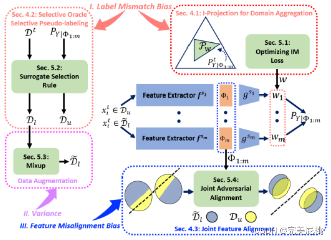

Domain aggregation aims to combine knowledge from multiple source domains to improve the performance of the target model. Helps reduce bias caused by label mismatch between source and target domains. There are two main methods for domain aggregation in the context of unsupervised multi-source domain-free adaptation (MSFDA). One method is to uniformly weight the predictions from multiple source models , but this may not be the best choice because of the different sources. Domains may have varying transferability. Instead, consider a mixture distribution with non-negative domain weights , where the predictions of each source model are weighted differently. This approach can produce lower bias than using any single model and can benefit domain adaptation problems. Increasing the number of source models with optimal blending weights can further improve the performance of the target model.
Selective pseudo-labeling is a strategy in unsupervised multi-source passive domain adaptation (MSFDA) for generating pseudo-labels for a subset of target domain data. The purpose of this strategy is to adopt certain standards during the generation of pseudo labels to ensure that bounded labels do not match the bias while reducing the variance to balance the bias-variance trade-off in MSFDA. Selective pseudo-label generation : In MSFDA, the real label of the target domain is usually not available, so pseudo-labels need to be generated for training. Selective pseudo-labeling refers to generating pseudo-labels only for a subset of the target domain data, rather than performing this operation on all samples in the target domain. Label mismatch bias criterion : In order to ensure that the generated pseudo labels are consistent with the label distribution of the source domain data to some extent, a criterion P(Dl|Y) ≤ P(t|y) is introduced, where Dl represents the target domain data The label distribution of , t represents the source domain data. This criterion can be viewed as a matching measure to ensure that the distribution of pseudo-labels does not mismatch the source domain labels too much. Reduced label mismatch bias and variance : The main advantage of selective pseudo-labeling is that it reduces the trade-off between label mismatch bias (the inaccuracy of the pseudo-labels) and variance (the noise introduced by the pseudo-labels). By selectively generating pseudo labels only for high-confidence target samples, the variance of pseudo labels can be reduced, since these samples are more likely to have accurate pseudo labels, thus providing a more reliable training signal. Balancing trade-offs : This approach helps balance the trade-off between label mismatch bias and variance. It ensures that the target model is not unduly affected by noise or incorrect pseudo-labels, while still benefiting from additional training data.
Joint feature alignment refers to the process of aligning feature representations of multiple source and target domains in unsupervised multi-source passive domain adaptation (MSFDA). The purpose of this process is to reduce the feature misalignment bias caused by inconsistent feature representation distribution between the source and target domains. Feature misalignment bias refers to the difference between feature representations in different domains. This difference may lead to a degradation in the performance of the model on the target domain. Multi-source feature representation : In MSFDA, there are usually multiple source domains and a target domain. Each domain has its own feature representation, usually generated by deep neural networks or other feature extraction methods. These feature representations may differ in different domains. Feature alignment : In order to improve the performance of the model on the target domain, feature alignment needs to be used to reduce the feature misalignment between the source domain and the target domain. The goal of feature alignment is to make feature representations in different domains more similar or close. Joint feature alignment : Joint feature alignment refers to aligning feature representations of multiple source and target domains in a joint representation space. This means not only considering feature alignment between source domains, but also considering aligning the feature representation of the target domain with the source domain so that they are more consistent in the same representation space. Joint adversarial feature alignment loss : To achieve joint feature alignment, a loss function such as joint adversarial feature alignment loss can be used. This loss helps balance the bias and variance of the model, reduce feature misalignment bias, and improve the model's performance on the target domain. It usually includes adversarial training to ensure that feature representations are more consistent in the joint representation space.
I-projection for Domain Aggregation

I-projection is a technique for domain aggregation in unsupervised multi-source domain adaptation, which makes the feature distribution of different source domains consistent with the target source domain by minimizing the maximum mean difference (MMD) between different source domains. consistent. The I-projection method achieves this by iteratively updating the feature representation of the target domain based on the features of the source domain. There are two main steps: feature extraction and feature alignment. In feature extraction, the target model is used to extract the target domain and features; in feature alignment, the extracted target features are aligned with the source features using MMD. This bad luck helps reduce the distribution difference between the source and target domains, thereby improving domain adaptation performance.

Optimizing IM Loss: The information maximizing loss estimated by IM Loss is a loss function used in the context of unsupervised multi-source domain-free adaptation. It is optimized to encourage source models to make individually deterministic yet global predictions. The IM loss is calculated by maximizing the difference between the entropy of the predictions made by the source model and the entropy of the aggregated predictions. This encourages the source model to make different predictions while confirming a person's prediction, applying instant message loss to the labeled source data to avoid overconfident but incorrect pseudo-labels in the unlabeled target data. It helps reduce label mismatch bias and improve the performance of the target model in domain adaptation tasks.

Selective oracle Selective Pseudo-labeling

A selective oracle refers to an ideal scenario in unsupervised multi-source passive domain adaptation, where an oracle can be used to ensure that a subset of the labels contains only correctly pseudo-labeled data. But actually such an oracle is not available. To overcome the problem of selective oracle unavailability, an agent selection rule is proposed that involves a pseudo-label denoising technique for improving the quality of label distribution and a confidence level for selecting new data for pseudo-labeling Query strategy. Selective pseudo-labeling is a technique used for multi-source domain-free adaptation to assign pseudo-labels to subsets of target data. It aims to balance the trade-off between bias and variance by selectively assigning pseudo-labels to subsets of data.

Agent selection rules, including pseudo-label denoising and confidence query strategies, help achieve selective unlabeling without the need for selective oracles. Pseudo-label denoising refers to the process of reducing noise in pseudo-labels assigned to target data in unsupervised multi-source passive domain adaptation. This is crucial because the source model's predictions on the target data can be very confusing, and various techniques, such as prototype-based pseudo-label denoising, can be used to improve the quality of the pseudo-labels. The confidence query strategy is used to select new data for pseudo-labels in multi-source domain-free adaptation. These strategies aim to identify the most confident samples, which can be more accurately assigned pseudo-labels. By selecting samples with higher confidence, the quality of the pseudo-labels can be improved, thereby improving the adaptation performance.

Joint Feature Alignment

Joint feature alignment is a technique for unsupervised multi-source domain-free adaptation to align feature representations of labeled source data and unlabeled target data in a joint representation space. Its goal is to reduce the feature misalignment bias caused by multiple source models in the joint representation space; it involves enforcing feature alignment between labeled source data and unlabeled target data in the joint representation space.

Joint adversarial feature alignment is a specific method for joint feature alignment, where a joint feature representation is constructed by combining features from each source model. A separate neural network is trained as a joint discriminator to distinguish joint features of labeled source data and unlabeled target data. Multiple feature extractors are updated together to fool a single discriminator, thereby achieving feature alignment.

Experimental results

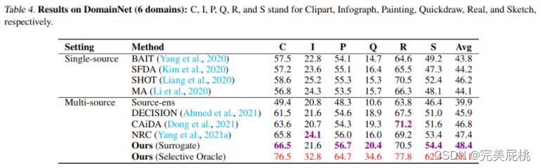
This study uses four benchmark datasets, namely Digits-Five, Office-31, Office-Home and DomainNet, to evaluate the performance of the proposed method. Digits-Five contains five different domain names, including MNIST, SVHN, USPS, MNIST-M, and synthetic digits, while Office-31 contains 31 categories collected from three different office environments, including Amazon, Webcam, and Digital SLR camera. Office-Home is a more challenging dataset, containing 65 categories collected from four different office environments, including art, clipart, real world, and products. DomainNet is the largest and most challenging domain name adaptation benchmark, containing approximately 600,000 images collected from six different domains, divided into 345 categories, including Clip Art, Infograph, Painting, Quickdraw, Real, and Sketch.

To demonstrate the empirical performance of the proposed method, this study compares it with recently proposed state-of-the-art (SOTA) multi-source domain adaptation methods including DECISION, CaidA, and NRC. The study also includes a baseline that evaluates the ensemble prediction accuracy of the target domain using pretrained source models (denoted as Source-ens). Furthermore, the study compares the performance of the proposed method with several SOTA passive domain adaptation methods including BAIT, SFDA, SHOT and MA. These single-source methods also do not require access to source data, and this study compares their multi-source ensemble results by taking the average of predictions from multiple retrained source models after adaptation.

Mixup data augmentation is a technique used to increase the diversity of training data and improve model generalization performance. It is a data augmentation strategy that is commonly used in the training of deep learning models, especially in image classification and deep learning tasks. The main idea of Mixup is to linearly mix the features and labels of two or more training samples to generate a new sample, thereby expanding the training data set .

Here are the key takeaways from Mixup data augmentation:

Mixed sample generation : For each pair of training samples, Mixup first randomly selects two samples (or multiple samples), and then linearly mixes their features and labels with a random weight factor. Typically, this weighting factor is uniformly randomly sampled within the interval [0, 1].
Feature Mixing : For two samples A and B, feature mixing is performed in the following way:

pythonCopy code Mixed_Feature = lambda * Feature_A + (1 - lambda) * Feature_B

Here, Mixed_Featureare the generated mixed features, Feature_Aand Feature_Bare the features of the two samples, and lambdaare the random weighting factors.

Label Mixing : Mixup also mixes labels, which is commonly used in classification tasks. For classification tasks, label blending is performed in the following way:

pythonCopy code Mixed_Label = lambda * Label_A + (1 - lambda) * Label_B

Here, Mixed_Labelis the generated hybrid label, Label_Aand Label_Bare the labels of the two samples.

Loss function : During training, the features of the mixed samples are used for forward propagation and the loss is calculated using the mixed labels. Typically, cross-entropy loss or other appropriate loss function is used to measure the difference between the model's predictions and the mixed labels.
Advantages : Mixup data enhancement helps reduce the risk of overfitting of the model, improves the generalization performance of the model, increases the diversity of training data, and also improves the robustness of the model to inputs. Mixup data augmentation has been widely used in deep learning tasks, especially in the field of image classification. It is a simple and effective regularization technique that helps improve the performance of the model, especially on small data sets.

5. Integrated learning

Ensemble learning is a technique that improves generalization performance by combining predictions from multiple models. Its core idea is to reduce the uncertainty and bias of a single model by combining the opinions of multiple models, thereby obtaining stronger generalization performance.

Reducing variance : Ensemble learning can reduce the variance of a model by combining multiple models together. A single model may overfit on the training data, resulting in high variance, but by integrating multiple different models, their overfitting tendencies may be different and therefore the overall variance can be reduced. This makes the ensemble model generalize better to new data.
Reduce bias : Ensemble learning also helps reduce bias in the model. A single model may be too simple to capture the complex relationships in the data, resulting in large biases. By combining the predictions of multiple models, the shortcomings of a single model can be compensated and the overall bias can be reduced.
Reduce the risk of overfitting : Because ensemble models are composed of multiple models, they are less prone to overfitting than individual models. If a model performs poorly on some data, other models may provide better predictions, reducing the risk of overfitting.
Increase diversity : The effectiveness of ensemble learning lies in the diversity among models. If there is enough differentiation between the ensemble's models, when one model makes a mistake, the other models may correct it. This diversity helps improve the generalization performance of the ensemble model.
Voting or averaging mechanism : In ensemble learning, a voting or averaging mechanism is often employed to combine the predictions of multiple models. This means that each model contributes a weight to the final prediction. This method can effectively aggregate the opinions of each model and improve the overall prediction performance. ★
Combination of different algorithms : Ensemble learning can also combine models of different algorithms, such as decision trees, support vector machines, neural networks, etc. Such a combination can make full use of the advantages of different algorithms, thereby improving generalization performance.

6. Model distillation

Model Distillation is a technology used to improve model generalization performance. Its main idea is to transfer the knowledge of a large, complex model to a small, simplified model, thereby realizing the migration and improvement of model performance. Generalizability.

Reduce model complexity : Typically, large deep neural networks have high complexity and number of parameters, and they are prone to overfitting on the training data. Small models (called student models) are relatively simple, have fewer parameters, and generalize more easily to new, unseen data. Through model distillation, the complexity of a large model can be transferred to a small model, helping the small model better capture patterns in the data.
Transfer model knowledge : In model distillation, the predictions and probability distributions of a large model (called a teacher model) are used to guide a small model. The teacher model has been trained on large-scale data, so it has more knowledge and generalization capabilities. Small models can gain this knowledge by learning the predictions of the teacher model, thereby improving generalization performance.
Soft Labels : In model distillation, the output of the teacher model is usually regarded as "soft labels". These soft labels are probability distributions rather than hard category labels. By comparing the soft labels of the teacher model, the student model can better learn the distribution and uncertainty of the data, thereby improving generalization performance.
Temperature Parameter : There is usually a temperature parameter in model distillation, which is used to control the "smoothness" of the distribution of soft labels. Appropriately adjusting the temperature parameters can help the student model better learn the knowledge of the teacher model, thereby improving generalization performance.
Regularization effect : Model distillation also has a regularization effect, which can reduce the risk of overfitting of the student model. By comparing with the teacher model, the student model prefers to learn categories with high probability rather than predicting a certain category with overconfidence.

7. Four ideas for scientific research in the era of large models

Four ideas for doing scientific research in the era of big models

Efficient(PEFT): Improve training efficiency, here we take PEFT (parameter efficient fine tuning) as an example
Existing stuff (pretrained model), New directions: Using other people’s pretrained models, new research directions
plug-and-play: Make some plug-and-play modules, such as model modules, objective functions, new loss functions, data enhancement methods, etc.
Dataset, evaluation and survey: Construct data sets and publish analysis-focused articles or review papers.

8. Resource Organization

Open source domain generalization library

https://github.com/jindongwang/transferlearning/tree/master/code/DeepDG

https://github.com/junkunyuan/Awesome-Domain-Generalization