Image recognition of crop diseases and insect pests based on convolutional neural network (Opencv, Pytorch, Tensorflow, MobileNetV3)

Foreword:

I recently made a program for image recognition of crop pests, and I would like to share it here. The deep learning frameworks used in this article are Tensorflow2, Opencv, etc.! The data set used has a total of 61 categories, representing different pest categories. The network model used is moblienetv3.

Bi 设 Dai za

The effect video is as follows:

Crop pest image recognition

Build mobilenetv3 model

The code looks like this:

# 根据tf.keras的官方代码修改的mobilenetv3的网络模型
import tensorflow as tf
from keras import layers, models

"""
    Reference:
    - [Searching for MobileNetV3](https://arxiv.org/pdf/1905.02244.pdf) (ICCV 2019)
    The following table describes the performance of MobileNets v3:
    ------------------------------------------------------------------------
    MACs stands for Multiply Adds
    |Classification Checkpoint|MACs(M)|Parameters(M)|Top1 Accuracy|Pixel1 CPU(ms)|
    |---|---|---|---|---|
    | mobilenet_v3_large_1.0_224              | 217 | 5.4 |   75.6   |   51.2  |
    | mobilenet_v3_large_0.75_224             | 155 | 4.0 |   73.3   |   39.8  |
    | mobilenet_v3_large_minimalistic_1.0_224 | 209 | 3.9 |   72.3   |   44.1  |
    | mobilenet_v3_small_1.0_224              | 66  | 2.9 |   68.1   |   15.8  |
    | mobilenet_v3_small_0.75_224             | 44  | 2.4 |   65.4   |   12.8  |
    | mobilenet_v3_small_minimalistic_1.0_224 | 65  | 2.0 |   61.9   |   12.2  |
    For image classification use cases, see
    [this page for detailed examples](https://keras.io/api/applications/#usage-examples-for-image-classification-models).
    For transfer learning use cases, make sure to read the
    [guide to transfer learning & fine-tuning](https://keras.io/guides/transfer_learning/).
"""


##################################################################################################################################
# 定义V3的完整模型 #################################################################################################################
##################################################################################################################################
def MobileNetV3(input_shape=[224, 224, 3], classes=1000, dropout_rate=0.2, alpha=1.0, weights=None,
                model_type='large', minimalistic=False, classifier_activation='softmax', include_preprocessing=False):
    # 如果有权重文件，那就意味着要迁移学习，那就意味着需要让BN层始终处于infer状态，否则解冻整个网络后，会出现acc下降loss上升的现象，终其原因是解冻网络之
    # 前，网络BN层用的是之前数据集的均值和方差，解冻后虽然维护着新的滑动平均和滑动方差，但是单次训练时使用的是当前batch的均值和方差，差异太大造成特征崩塌
    if weights:
        bn_training = False
    else:
        bn_training = None
    bn_decay = 0.99  # BN层的滑动平均系数，这个值的设置需要匹配steps和batchsize否则会出现奇怪现象
    # 确定通道所处维度
    channel_axis = -1
    # 根据是否为mini设置，修改部分配置参数
    if minimalistic:
        kernel = 3
        activation = relu
        se_ratio = None
        name = "mini"
    else:
        kernel = 5
        activation = hard_swish
        se_ratio = 0.25
        name = "norm"
    # 定义模型输入张量
    img_input = layers.Input(shape=input_shape)
    # 是否包含预处理层
    if include_preprocessing:
        x = layers.Rescaling(scale=1. / 127.5, offset=-1.)(img_input)
    else:
        x = img_input
    # 定义整个模型的第一个特征提取层
    x = layers.Conv2D(16, kernel_size=3, strides=(2, 2), padding='same', use_bias=False, name='Conv')(x)
    x = layers.BatchNormalization(axis=channel_axis, epsilon=1e-3, momentum=bn_decay, name='Conv/BatchNorm')(x,
                                                                                                             training=bn_training)
    x = activation(x)
    # 定义整个模型的骨干特征提取
    if model_type == 'large':
        x = MobileNetV3Large(x, kernel, activation, se_ratio, alpha, bn_training, bn_decay)
        last_point_ch = 1280
    else:
        x = MobileNetV3Small(x, kernel, activation, se_ratio, alpha, bn_training, bn_decay)
        last_point_ch = 1024
    # 定义整个模型的后特征提取
    last_conv_ch = _depth(x.shape[channel_axis] * 6)
    # if the width multiplier is greater than 1 we increase the number of output channels
    if alpha > 1.0:
        last_point_ch = _depth(last_point_ch * alpha)
    x = layers.Conv2D(last_conv_ch, kernel_size=1, padding='same', use_bias=False, name='Conv_1')(x)
    x = layers.BatchNormalization(axis=channel_axis, epsilon=1e-3, momentum=bn_decay, name='Conv_1/BatchNorm')(x,
                                                                                                               training=bn_training)
    x = activation(x)
    # 如果tf版本大于等于2.6则直接使用下面第一句就可以了，否则使用下面2~3句
    # x = layers.GlobalAveragePooling2D(data_format='channels_last', keepdims=True)(x)
    x = layers.GlobalAveragePooling2D(data_format='channels_last')(x)
    x = tf.expand_dims(tf.expand_dims(x, 1), 1)
    # 定义第一个特征分类层
    x = layers.Conv2D(last_point_ch, kernel_size=1, padding='same', use_bias=True, name='Conv_2')(x)
    x = activation(x)
    # 定义第二个特征分类层
    if dropout_rate > 0:
        x = layers.Dropout(dropout_rate)(x)
    x = layers.Conv2D(classes, kernel_size=1, padding='same', name='Logits')(x)
    x = layers.Flatten()(x)
    x = layers.Activation(activation=classifier_activation, name='Predictions')(x)  # 注意损失函数需要与初始权重匹配，否则预训练没有意义
    # 创建模型
    model = models.Model(img_input, x, name='MobilenetV3' + '_' + model_type + '_' + name)
    # 恢复权重
    if weights:
        model.load_weights(weights, by_name=True)
        # print(model.get_layer(name="block_8_project_BN").get_weights()[0][:4])

    return model


##################################################################################################################################
# 定义V3的骨干网络，不包含前处理和后处理 ###############################################################################################
##################################################################################################################################

# 定义mobilenetv3-small的骨干部分，不包含第一层的卷积特征提取和后处理
def MobileNetV3Small(x, kernel, activation, se_ratio, alpha, bn_training, mome):
    def depth(d):
        return _depth(d * alpha)

    x = _inverted_res_block(x, 1, depth(16), 3, 2, se_ratio, relu, 0, bn_training, mome)
    x = _inverted_res_block(x, 72. / 16, depth(24), 3, 2, None, relu, 1, bn_training, mome)
    x = _inverted_res_block(x, 88. / 24, depth(24), 3, 1, None, relu, 2, bn_training, mome)
    x = _inverted_res_block(x, 4, depth(40), kernel, 2, se_ratio, activation, 3, bn_training, mome)
    x = _inverted_res_block(x, 6, depth(40), kernel, 1, se_ratio, activation, 4, bn_training, mome)
    x = _inverted_res_block(x, 6, depth(40), kernel, 1, se_ratio, activation, 5, bn_training, mome)
    x = _inverted_res_block(x, 3, depth(48), kernel, 1, se_ratio, activation, 6, bn_training, mome)
    x = _inverted_res_block(x, 3, depth(48), kernel, 1, se_ratio, activation, 7, bn_training, mome)
    x = _inverted_res_block(x, 6, depth(96), kernel, 2, se_ratio, activation, 8, bn_training, mome)
    x = _inverted_res_block(x, 6, depth(96), kernel, 1, se_ratio, activation, 9, bn_training, mome)
    x = _inverted_res_block(x, 6, depth(96), kernel, 1, se_ratio, activation, 10, bn_training, mome)

    return x


# 定义mobilenetv3-large的骨干部分，不包含第一层的卷积特征提取和后处理
def MobileNetV3Large(x, kernel, activation, se_ratio, alpha, bn_training, mome):
    def depth(d):
        return _depth(d * alpha)

    x = _inverted_res_block(x, 1, depth(16), 3, 1, None, relu, 0, bn_training, mome)
    x = _inverted_res_block(x, 4, depth(24), 3, 2, None, relu, 1, bn_training, mome)
    x = _inverted_res_block(x, 3, depth(24), 3, 1, None, relu, 2, bn_training, mome)
    x = _inverted_res_block(x, 3, depth(40), kernel, 2, se_ratio, relu, 3, bn_training, mome)
    x = _inverted_res_block(x, 3, depth(40), kernel, 1, se_ratio, relu, 4, bn_training, mome)
    x = _inverted_res_block(x, 3, depth(40), kernel, 1, se_ratio, relu, 5, bn_training, mome)
    x = _inverted_res_block(x, 6, depth(80), 3, 2, None, activation, 6, bn_training, mome)
    x = _inverted_res_block(x, 2.5, depth(80), 3, 1, None, activation, 7, bn_training, mome)
    x = _inverted_res_block(x, 2.3, depth(80), 3, 1, None, activation, 8, bn_training, mome)
    x = _inverted_res_block(x, 2.3, depth(80), 3, 1, None, activation, 9, bn_training, mome)
    x = _inverted_res_block(x, 6, depth(112), 3, 1, se_ratio, activation, 10, bn_training, mome)
    x = _inverted_res_block(x, 6, depth(112), 3, 1, se_ratio, activation, 11, bn_training, mome)
    x = _inverted_res_block(x, 6, depth(160), kernel, 2, se_ratio, activation, 12, bn_training, mome)
    x = _inverted_res_block(x, 6, depth(160), kernel, 1, se_ratio, activation, 13, bn_training, mome)
    x = _inverted_res_block(x, 6, depth(160), kernel, 1, se_ratio, activation, 14, bn_training, mome)

    return x


##################################################################################################################################
# 定义V3的骨干模块 #################################################################################################################
##################################################################################################################################

# 定义relu函数
def relu(x):
    return layers.ReLU()(x)


# 定义sigmoid函数的近似函数h-sigmoid函数
def hard_sigmoid(x):
    return layers.ReLU(6.)(x + 3.) * (1. / 6.)


# 定义swish函数的近似函数，替换原本的sigmoid函数为新的h-sigmoid函数
def hard_swish(x):
    return layers.Multiply()([x, hard_sigmoid(x)])


# python中变量前加单下划线：是提示程序员该变量或函数供内部使用，但不是强制的，只是提示，但是不能用“from xxx import *”而导入
# python中变量后加单下划线：是避免变量名冲突
# python中变量前加双下划线：是强制该变量或函数供类内部使用，名称会被强制修改，所以原名称无法访问到，新名称可以访问到，所以也不是外部完全无法访问
# python中变量前后双下划线：是用于类内部定义使用，是特殊用途，外部可以直接访问，平时程序员不要这样定义
# 通过函数实现不管v为多大，输出new_v始终能够被divisor整除，且new_v是大于等于min_value且不能太小的四舍五入最接近divisor整除的数
def _depth(v, divisor=8, min_value=None):
    if min_value is None:
        min_value = divisor
    # 保证new_v一定大于等于min_value，max中第二个值保证是v的四舍五入的能够被divisor整除的数
    new_v = max(min_value, int(v + divisor / 2) // divisor * divisor)
    # 保证new_v不要太小
    if new_v < 0.9 * v:
        new_v += divisor
    return new_v


# 在stride等于2时，计算pad的上下左右尺寸，注:在stride等于1时，无需这么麻烦，直接就是correct，本函数仅仅针对stride=2
def pad_size(inputs, kernel_size):
    input_size = inputs.shape[1:3]
    if isinstance(kernel_size, int):
        kernel_size = (kernel_size, kernel_size)
    if input_size[0] is None:
        adjust = (1, 1)
    else:
        adjust = (1 - input_size[0] % 2, 1 - input_size[1] % 2)
    correct = (kernel_size[0] // 2, kernel_size[1] // 2)
    return ((correct[0] - adjust[0], correct[0]),
            (correct[1] - adjust[1], correct[1]))


# 定义通道注意力机制模块，这里filters数字应该是要等于inputs的通道数的，否则最后一步的相乘无法完成，se_ratio可以调节缩放比例
def _se_block(inputs, filters, se_ratio, prefix):
    # 如果tf版本大于等于2.6则直接使用下面第一句就可以了，否则使用下面2~3句
    # x = layers.GlobalAveragePooling2D(data_format='channels_last', keepdims=True, name=prefix + 'squeeze_excite/AvgPool')(inputs)
    x = layers.GlobalAveragePooling2D(data_format='channels_last', name=prefix + 'squeeze_excite/AvgPool')(inputs)
    x = tf.expand_dims(tf.expand_dims(x, 1), 1)
    x = layers.Conv2D(_depth(filters * se_ratio), kernel_size=1, padding='same', name=prefix + 'squeeze_excite/Conv')(x)
    x = layers.ReLU(name=prefix + 'squeeze_excite/Relu')(x)
    x = layers.Conv2D(filters, kernel_size=1, padding='same', name=prefix + 'squeeze_excite/Conv_1')(x)
    x = hard_sigmoid(x)
    x = layers.Multiply(name=prefix + 'squeeze_excite/Mul')([inputs, x])
    return x


# 定义V3的基础模块，可以通过expansion调整模块中所有特整层的通道数，se_ratio可以调节通道注意力机制中的缩放系数
def _inverted_res_block(x, expansion, filters, kernel_size, stride, se_ratio, activation, block_id, bn_training, mome):
    channel_axis = -1  # 在tf中通道维度是最后一维
    shortcut = x
    prefix = 'expanded_conv/'
    infilters = x.shape[channel_axis]
    if block_id:
        prefix = 'expanded_conv_{}/'.format(block_id)
        x = layers.Conv2D(_depth(infilters * expansion), kernel_size=1, padding='same', use_bias=False,
                          name=prefix + 'expand')(x)
        x = layers.BatchNormalization(axis=channel_axis, epsilon=1e-3, momentum=mome, name=prefix + 'expand/BatchNorm')(
            x, training=bn_training)
        x = activation(x)

    if stride == 2:
        x = layers.ZeroPadding2D(padding=pad_size(x, kernel_size), name=prefix + 'depthwise/pad')(x)
    x = layers.DepthwiseConv2D(kernel_size, strides=stride, padding='same' if stride == 1 else 'valid', use_bias=False,
                               name=prefix + 'depthwise')(x)
    x = layers.BatchNormalization(axis=channel_axis, epsilon=1e-3, momentum=mome, name=prefix + 'depthwise/BatchNorm')(
        x, training=bn_training)
    x = activation(x)

    if se_ratio:
        x = _se_block(x, _depth(infilters * expansion), se_ratio, prefix)

    x = layers.Conv2D(filters, kernel_size=1, padding='same', use_bias=False, name=prefix + 'project')(x)
    x = layers.BatchNormalization(axis=channel_axis, epsilon=1e-3, momentum=mome, name=prefix + 'project/BatchNorm')(x,
                                                                                                                     training=bn_training)

    if stride == 1 and infilters == filters:
        x = layers.Add(name=prefix + 'Add')([shortcut, x])
    return x
if __name__ == '__main__':
    mobilev3=MobileNetV3(input_shape=[64,64,3],classes=61)
    mobilev3.summary()

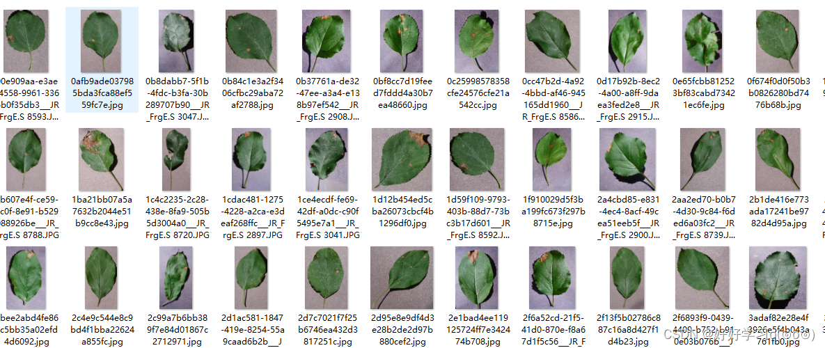
data set:

The data set contains a total of 61 crop images of different pest and disease categories, some of which are shown below.

Model training:

The training code looks like this:

import numpy as np
import tensorflow as tf
import keras
from model import MobileNetV3
import matplotlib.pyplot as plt

x_train=np.load('data/x_train.npy')
y_train=np.load('data/y_train.npy')
x_val=np.load('data/x_val.npy')
y_val=np.load('data/y_val.npy')

#归一化
x_train=(x_train/255.0).astype('float32')
x_val=(x_val/255.0).astype('float32')

model=MobileNetV3(input_shape=[64,64,3],classes=61)
# model.compile() 优化器、损失函数和准确率评测标准
model.compile(optimizer='adam',
              loss=tf.keras.losses.SparseCategoricalCrossentropy(from_logits=False),
              metrics=['accuracy'])

history = model.fit(x_train, y_train, epochs=50,batch_size=128, validation_data=(x_val, y_val))
model.save('model.h5')

acc = history.history['accuracy']
val_acc = history.history['val_accuracy']
loss = history.history['loss']
val_loss = history.history['val_loss']

plt.subplot(1, 2, 1)
plt.plot(acc, label='Training Accuracy')
plt.plot(val_acc, label='Validation Accuracy')
plt.title('Training and Validation Accuracy')
plt.legend()

plt.subplot(1, 2, 2)
plt.plot(loss, label='Training Loss')
plt.plot(val_loss, label='Validation Loss')
plt.title('Training and Validation Loss')
plt.legend()
plt.savefig('acc_loss.png')
plt.show()

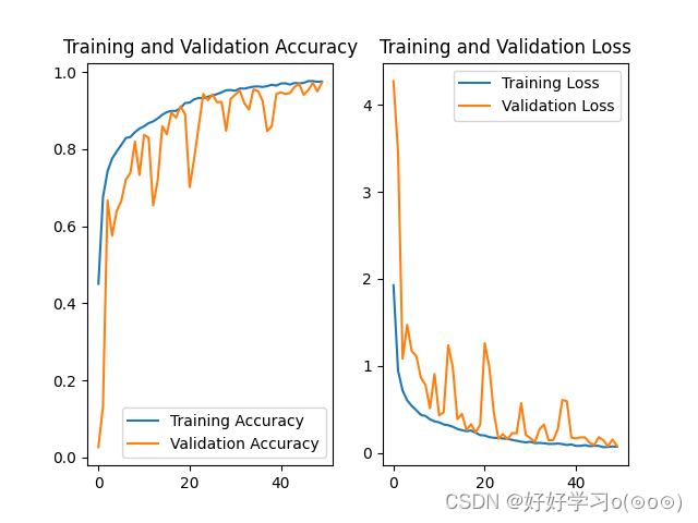
Loss plot and accuracy image:

As can be seen from the figure below, the effect of the model is still acceptable.

Project download:

The project structure is as follows:

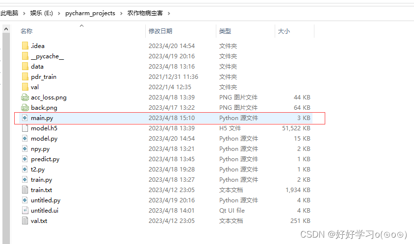
Run main.py to pop up the interface window, as shown below:

Project download:Project download