July is too busy, let's write an article!
Welcome to "Python from Zero to One", where I will share about 200 Python series articles, take everyone to learn and play together, and see the interesting world of Python. All articles will be explained in combination with cases, codes and the author's experience. I really want to share my nearly ten years of programming experience with you. The overall framework of the Python series includes 10 articles on basic grammar, 30 articles on web crawlers, 10 articles on visual analysis, 20 articles on machine learning, 20 articles on big data analysis, 30 articles on image recognition, 40 articles on artificial intelligence, 20 articles on Python security, and 10 articles on other skills. Your attention, likes and retweets are the greatest support for Xiuzhang. Knowledge is priceless. I hope we can all be happy and grow together on the road of life.
This series of articles mainly explains the knowledge of Python OpenCV image processing and image recognition. In the early stage, it mainly explains the basic knowledge of image processing, basic usage of OpenCV, common image drawing methods, image geometric transformation, etc. In the middle stage, it explains various operations of image processing, including image point operations, morphological processing, image sharpening, image enhancement, image smoothing, etc., and later researches image recognition, image segmentation, image classification, image special effects processing, and image processing related applications.
In the first part, the author introduces the basics of image processing. In the second part, image computing and image enhancement are introduced. In the next part, we will explain in detail the classic cases of image recognition and image processing. This part belongs to advanced image processing knowledge, which can further deepen our understanding and practical ability. Image classification is an image processing method that distinguishes different types of objects according to the different characteristics reflected in the image information. The previous article mainly explained the common image classification algorithms, and introduced the Bayesian image classification algorithm in the Python environment and the image classification based on the KNN algorithm. This article will use convolutional neural networks to implement MNIST (handwritten digits) image classification, which is also a classic image classification case. I hope the article is helpful to you, if there are any deficiencies, please forgive me.
Article Directory
Download URL: Remember to like it O(∩_∩)O
- https://github.com/eastmountyxz/Python-zero2one
- Open source e-book with more than 600 pages: https://github.com/eastmountyxz/HWCloudImageRecognition
Appreciation of the previous article: (Although this part takes up a lot of space, I am reluctant to delete it, haha!)
Part I Basic Grammar
- [Python from zero to one] 1. Why we should learn Python and basic grammar
- [Python from zero to one] 2. Conditional statements, loop statements and functions on the basis of grammar
- [Python from zero to one] 3. File operations based on grammar, CSV file reading and writing and object-oriented
Part II Web Crawlers
- [Python from zero to one] 4. The basics of getting started with web crawlers and the case of blog crawling with regular expressions
- [Python from zero to one] Five. Detailed explanation of the basic grammar of BeautifulSoup for web crawlers
- [Python from zero to one] Six. BeautifulSoup of web crawler crawls Douban TOP250 movies in detail
- [Python from zero to one] 7. Requests of web crawlers crawl Douban movie TOP250 and CSV storage
- [Python from zero to one] 8. Basic knowledge and operation of MySQL database in detail
- [Python from zero to one] 9. Detailed explanation of Selenium basic technology of web crawler (positioning elements, common methods, keyboard and mouse operations)
- [Python from zero to one] 10. Selenium of web crawlers crawls online encyclopedia knowledge in detail (necessary skills for NLP corpus construction)
Part III Data Analysis and Machine Learning
- [Python from zero to one] Eleven. Data analysis of Numpy, Pandas, Matplotlib and Sklearn introductory knowledge ten thousand word detailed explanation (1)
- [Python from zero to one] 12. Regression analysis of machine learning 4-word summary first published on the whole network (linear regression, polynomial regression, logistic regression)
- [Python from zero to one] Thirteen. Cluster analysis of machine learning 4 word summary first launch on the whole network (K-Means, BIRCH, hierarchical clustering, tree clustering)
- [Python from zero to one] 14. The 30,000-word summary of the classification algorithm of machine learning is first published on the whole network (comparison of decision tree, KNN, SVM, and classification algorithm)
- [Python from zero to one] 15. Detailed explanation of data preprocessing, Jieba tools and text clustering for text mining
- [Python from zero to one] 16. Detailed explanation of word cloud hotspots and LDA topic distribution analysis of text mining
- [Python from zero to one] 17. Detailed explanation of Matplotlib, Pandas, Echarts entry for visual analysis
- [Python from zero to one] Eighteen. Detailed introduction to the Basemap map package for visual analysis
- [Python from zero to one] Nineteen. Visual analysis of heat map and box plot drawing and application details
- [Python from zero to one] 20. Detailed explanation of Seaborn drawing for visual analysis
- [Python from zero to one] 21. Detailed explanation of Pyechart drawing for visual analysis
- [Python from zero to one] 22. Detailed explanation of OpenGL drawing for visual analysis
- [Python from zero to one] 23. Detailed explanation of decision tree classification analysis of top ten machine learning algorithms (1)
- [Python from zero to one] 24. Detailed explanation of KMeans cluster analysis of top ten machine learning algorithms (2)
- [Python from zero to one] 25. KNN algorithm and image classification of top ten machine learning algorithms (3)
- [Python from zero to one] 26. Naive Bayesian algorithm and text classification of top ten machine learning algorithms (4)
- [Python from zero to one] 27. Detailed analysis of linear regression algorithm of top ten machine learning algorithms (5)
- [Python from zero to one] Twenty-eight. Detailed analysis of the SVM algorithm of the top ten machine learning algorithms (6)
- [Python from zero to one] 29. Detailed analysis of random forest algorithm of top ten machine learning algorithms (7)
- [Python from zero to one] Thirty. Logistic regression algorithm of top ten machine learning algorithms and detailed explanation of malicious request detection application (8)
- [Python from zero to one] 31. Detailed explanation of Boosting and AdaBoost application of top ten machine learning algorithms (9)
- [Python from zero to one] Thirty-two. Detailed explanation of hierarchical clustering and dendrogram clustering application of top ten machine learning algorithms (10)
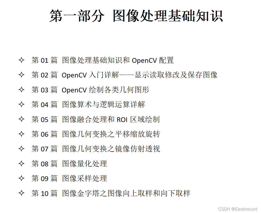
Part IV Basics of Python Image Processing
- [Python from zero to one] Thirty-three. Image processing basics: what is image processing and OpenCV configuration
- [Python from zero to one] Thirty-four. Detailed introduction to OpenCV - display, read, modify and save images
- [Python from zero to one] Thirty-five. OpenCV draws various geometric figures in the basics of image processing
- [Python from zero to one] Thirty-six. Detailed explanation of image arithmetic and logic operations in the basics of image processing
- [Python from zero to one] Thirty-seven. Image fusion processing and ROI area drawing in the basics of image processing
- [Python from zero to one] Thirty-eight. Image geometric transformation of image processing basics (translation, zoom and rotation)
- [Python from zero to one] Thirty-nine. Image geometric transformation of image processing basics (mirror affine perspective)
- [Python from zero to one] 40. Image quantization processing of image processing basics
- [Python from zero to one] 41. Image sampling processing of image processing basics
- [Python from zero to one] 42. Image pyramid upsampling and downsampling in image processing basics
Part V Python image operation and image enhancement
- [Python from zero to one] Forty-three. Image point operation and image grayscale processing of image enhancement and operation
- [Python from zero to one] 44. Detailed explanation of image grayscale linear transformation in image enhancement and operation
- [Python from zero to one] 45. Detailed explanation of image grayscale nonlinear transformation in image enhancement and operation
- [Python from zero to one] Forty-six. Image thresholding processing of image enhancement and operation
- [Python from zero to one] Forty-seven. Detailed explanation of corrosion and expansion of image enhancement and calculation
- [Python from zero to one] Forty-eight. Morphological opening operation, closing operation and gradient operation of image enhancement and operation
- [Python from zero to one] Forty-nine. Top-hat operation and bottom-hat operation of image enhancement and operation
- [Python from zero to one] 50. Theoretical knowledge and drawing realization of image histogram in image enhancement and operation
- [Python from zero to one] Fifty-one. Image enhancement and calculation of the image gray histogram comparison analysis Wanzi detailed explanation
- [Python from zero to one] 52. Image mask histogram and HS histogram of image enhancement and calculation
- [Python from zero to one] Fifty-three. Histogram equalization processing of image enhancement and calculation
- [Python from zero to one] 54. Local histogram equalization and automatic color equalization processing of image enhancement and calculation
- [Python from zero to one] 55. Image smoothing in image enhancement and calculation (mean filtering, box filtering, Gaussian filtering)
- [Python from zero to one] 56. Image smoothing in image enhancement and calculation (median filter, bilateral filter)
- [Python from zero to one] Fifty-seven. Image enhancement and operation chapter image sharpening Roberts, Prewitt operator to achieve edge detection
- [Python from zero to one] Fifty-eight. Image enhancement and operation chapter image sharpening Sobel, Laplacian operator to achieve edge detection
- [Python from zero to one] Fifty-nine. Image enhancement and calculation of image sharpening Scharr, Canny, LOG to achieve edge detection
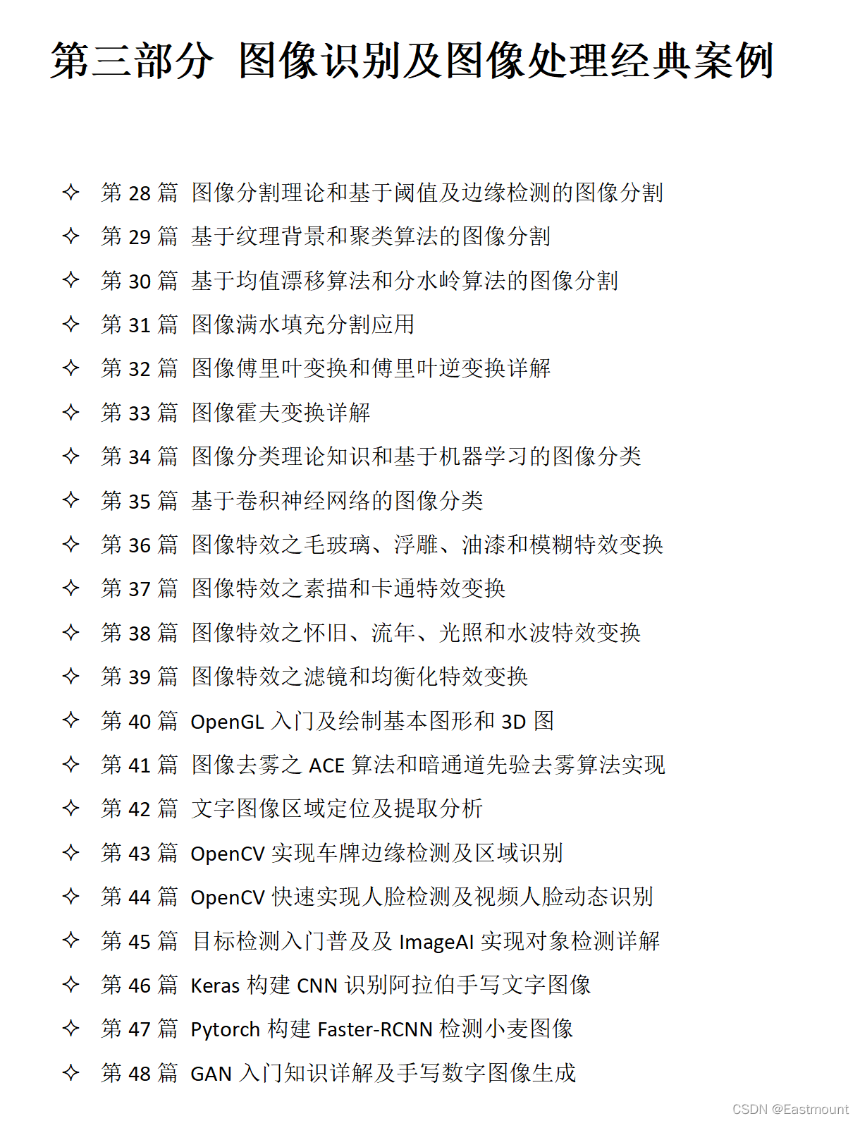
Part VI Python image recognition and high-level image cases
- [Python from zero to one] 60. Image segmentation based on threshold and edge detection in image recognition and classic cases
- [Python from zero to one] 61. Image recognition and classic cases: image segmentation based on texture background and clustering algorithm
- [Python from zero to one] 62. Image Recognition and Classic Cases: Image Segmentation Based on Mean Shift Algorithm and Watershed Algorithm
- [Python from zero to one] 63. Image recognition and classic cases of image flood filling segmentation application
- [Python from zero to one] Sixty-four. Detailed explanation of image Fourier transform and inverse Fourier transform of image recognition and classic cases
- [Python from zero to one] 65. Detailed explanation of image Hough transform in image recognition and classic cases
- [Python from zero to one] 66. Image classification based on machine learning in image recognition and classic cases
- [Python from zero to one] Sixty-seven. Image recognition and classic cases: MNIST image classification based on convolutional neural network
Part VII NLP and Text Mining
Part VIII Introduction to Artificial Intelligence
Part IX Network Attack and Defense and AI Security
The tenth part knowledge map construction practice
Extend some advanced cases of artificial intelligence
The author's newly opened "Nazhang AI Security Home" will focus on Python and security technology, mainly sharing articles on web penetration, system security, artificial intelligence, big data analysis, image recognition, malicious code detection, CVE recurrence, threat intelligence analysis, etc. Although the author is a technical novice, he will ensure that every article will be written with great care. I hope these basic articles will help you and make progress with everyone on the road of Python and security.
1. Image classification
Image classification (Image Classification) is the problem of classifying image content. It uses computers to quantitatively analyze images, and divides images or areas in images into several categories to replace human visual judgment. The traditional method of image classification is feature description and detection. This kind of traditional method may be effective for some simple image classification, but due to the complexity of the actual situation, the traditional classification method is overwhelmed. Now, machine learning and deep learning methods are widely used to deal with image classification problems. The main task is to assign a bunch of input pictures to a certain label in a known mixed category.
In Figure 1, the image classification model will take a single image and will assign corresponding probabilities {0.6, 0.3, 0.05, 0.05} to 4 labels {cat, dog, hat, mug}, where 0.6 represents the probability that the image label is a cat, and the rest are analogous. As shown, the image is represented as a three-dimensional array. In this example, the cat image has a width of 248 pixels and a height of 400 pixels, and has three color channels of red, green and blue (commonly referred to as RGB). Therefore, the image consists of 248x400x3 numbers or a total of 297600 numbers, each number being an integer from 0 (black) to 255 (white). The task of image classification is to turn these close to 300,000 numbers into a single label, such as "cat".

So, how do you write an algorithm for image classification? And how to identify a cat from many images? The method adopted here is similar to teaching children to look at pictures and recognize objects. Given a lot of image data, let the model continuously learn the characteristics of each class. Before training, it is first necessary to classify and label the images in the training set, as shown in Figure 2, including four categories: cat, dog, mug, and hat. In actual engineering, there may be thousands of categories of objects, and each category will have millions of images.

Image classification is to input an array of pixel values of a bunch of images, and then assign a classification label to it, build an algorithm model through training and learning, and then use the model to predict image classification. The image classification process based on the neural network is shown in Figure 35-3, refer to the sharing by the teacher of the NetEase cloud course "Mofan".
As shown in the figure below, generally speaking, the things processed by computers are different from those of humans. Whether it is sound, pictures or text, they can only appear in the computer neural network as numbers 0 or 1. The pictures seen by the neural network are actually a bunch of numbers, and the processing of the numbers will eventually generate another bunch of numbers, which have certain cognitive significance. Through a little bit of processing, we can know whether the computer judges whether the picture is a cat or a dog.

Classification belongs to a category of supervised learning, which is an important research field in data mining, machine learning and data science. The classification model is similar to the way humans learn. An objective function is obtained by learning historical data or training sets, and then the objective function is used to predict unknown attributes of new data sets. The classification model mainly consists of two steps:
- training . Given a data set, each sample contains a set of features and a category information, and then call the classification algorithm to train the model.
- predict . Use the generated model to classify and predict the new data set (test set), and judge its classification results.
Usually, a validation set is used to test the performance of the learned model. The data set will be divided into disjoint training set and test set, the training set is used to construct the classification model, and the test set is used to check how many class labels are correctly classified.
2. Neural network
Neural Network (Neural Network) is a classification method for non-linearly separable data, usually including an input layer, a hidden layer and an output layer. Among them, the layer directly connected to the input is called the hidden layer (Hidden Layer), and the layer directly connected to the output is called the output layer (Output Layer). The characteristic of the neural network algorithm is that there are more local optimal values, and the optimal value can be obtained by randomly setting the initial value multiple times and running the gradient descent algorithm. The most widely used in image classification are BP neural network and CNN neural network.
BP neural network is a multi-layer feed-forward neural network, its main characteristics are: the signal is propagated forward, and the error is propagated backward. The process of the BP neural network is mainly divided into two stages. The first stage is the forward propagation of the signal, from the input layer to the hidden layer, and finally reaches the output layer; the second stage is the backpropagation of the error, from the output layer to the hidden layer, and finally to the input layer. The weight and bias from the hidden layer to the output layer, and the weight and bias from the input layer to the hidden layer are adjusted in turn. The specific structure is shown in Figure 4.

The basic building block of a neural network is a neuron. The general model of neurons is shown in Figure 5, where commonly used activation functions include threshold function, sigmoid function, and hyperbolic tangent function.

The output of the neuron is:

3. Convolutional neural network
Convolutional Neural Networks (Convolutional Neural Networks) is a type of feed-forward neural network that includes convolution calculations and has a deep structure. It is one of the representative algorithms for deep learning. Research on convolutional neural networks began in the 1980s and 1990s, and time-delay networks and LeNet-5 were the earliest convolutional neural networks. After the 21st century, with the introduction of deep learning theory and the improvement of numerical computing equipment, convolutional neural networks have developed rapidly and have been widely used in computer vision, natural language processing and other fields.

Figure 6 is a CNN model for recognition. The leftmost picture is the two-dimensional matrix of the input layer, and then the convolutional layer. The activation function of the convolutional layer uses ReLU, ie. After the convolutional layer is the pooling layer, which and the convolutional layer are unique to CNN, and there is no activation function in the pooling layer. The combination of convolutional layer and pooling layer can appear many times in the hidden layer. In the above figure, the cycle appears twice, but in fact this number is determined according to the needs of the model. The common CNN is a combination of several convolutional layers and pooling layers. Behind several convolutional layers and pooling layers is a fully connected layer. The final output layer uses the Softmax activation function for image recognition classification.
The neural network is composed of many neural layers. There are many neurons in each layer of neural layers. These neurons are the key to identifying things. When the input is a picture, it is actually a bunch of numbers. Convolution means that instead of processing each pixel, it processes the image area. This method strengthens the continuity of the image and sees a graph instead of a point, which also deepens the neural network's understanding of the image.
The following is a detailed introduction to the principle knowledge of CNN in combination with the Google recommended video.
Suppose you have a photo of a kitten, as shown in the figure below, it can be represented as a pancake, it has width (width) and height (height), and because of the natural existence of red, green and blue, it also has RGB thickness (depth), at this time your input depth is 3.

Suppose we now take a small piece of the picture, run a small neural network with K outputs, and represent the output as a small vertical column as in the figure.

Without changing the weight, the small neural network slides through the entire picture, just like we slide horizontally and vertically with a brush to paint the wall.

At this point, another image is drawn at the output, as shown in the red area in the figure below. It is different from the previous width and height, and more importantly, it is different from the previous depth, instead of just red, green and blue, now you get K color channels, this operation is called——convolution。

If your block size is the whole image, it's no different than a normal neural network layer, just because we use small blocks, we have many small blocks that share less weight in space. Convolution does not process each pixel, but processes the image area. This approach strengthens the continuity of the image and deepens the neural network's understanding of the image.

A convolutional network is the basis for forming a deep network, and we will use several layers of convolutions instead of several layers of matrix multiplication. As shown in the figure below, let it form a pyramid shape. The bottom of the pyramid is a very large and shallow picture, including only red, green and blue. The dimension of the space is gradually squeezed through the convolution operation, and the depth is continuously increased, so that the depth information can basically represent complex semantics. At the same time, you can implement a classifier at the top of the pyramid. All spatial information is compressed into a logo, and only the information that maps pictures to different classes is retained. This is the general idea of CNN.
The specific process of the above figure is as follows:
- First of all, this is a color picture, which includes RGB three primary color components. The length and width of the image are 256x256, and the three layers correspond to the red (R), green (G), and blue (B) layers, which can also be regarded as the thickness of pixels.
- Secondly, CNN compresses the length and width of the picture into a 128x128x16 square. The compression method is to reduce the length and width of the picture to increase the thickness.
- Again, continue to compress to 64x64x64, until 32x32x256, at this time it becomes a very thick long square, which we call the classifier Classifier here. The classifier can predict our classification results. The prediction result of the MNIST handwritten data set is 10 numbers, such as [0,0,0,1,0,0,0,0,0,0] means that the predicted result is the number 3, and the Classifier here is equivalent to these 10 sequences.
- Finally, CNN continuously compresses the length and width of the picture, increases the thickness, and eventually becomes a very thick classifier for classification prediction.
If you want to implement it, there are many details that must be implemented correctly. At this point, you have come into contact with the concept of block and depth. A block (PATCH) is sometimes called a kernel (KERNEL). As shown in the figure below, each pancake in your stack is called a feature map (Feature Map). Here, three features are mapped to K feature maps. The function of PATCH/KERNEL is to extract a small part from the picture for analysis. Each small part extracted will become a sequence of length, width, and K thickness.

Another concept you need to know is - stride (STRIDE). It's the amount of pixels to translate when you move the filter or decimation, and how many steps are taken each time to decimate pixels in the image.

If the stride is equal to 1, it means that every time a pixel is pulled away, the resulting size is basically the same as the input.

If the stride STRIDE is equal to 2, it means that it is drawn away by 2 pixels each time, which means that it becomes half the size. The information it collects is reduced, the length and width of the picture are compressed, and the compression is merged into a smaller cube.

After compression, it is merged into a cube, which is a smaller cube that contains all the information in the picture.

The method of extracting image information is called PADDING (filling), which is generally divided into two types:
- VALID PADDING : The extracted layer is a bit wider and longer than the original image, and the extracted content is all in the image.
- SAME PADDING : The extracted layer has the same length and width as the previous image, and the extracted content is outside the image, and the value outside the image is filled with 0.

Research has found that some information will be lost during the convolution process. For example, if you want to take two steps to extract important information from the original image to form an image with a smaller length and width, important image information may be lost during this process. In order to solve this problem, it can be avoided by POOLING. The method is: no longer compress the length and width during convolution, try to ensure more information, and leave the compression work to POOLING. After the picture is convolved, the convolution information is processed by convolution, and then convolution is carried out again, and the result is passed to two layers of fully connected neural layers, and finally the cat or dog is identified through the classifier.

Summary: The entire CNN goes through the process of "picture->convolution->persistence->convolution->persistence->results are transferred to two layers of fully connected neural layers->classifier" from bottom to top, and finally realizes the classification process of a CNN.
- IMAGE picture
- CONVOLUTION layer
- MAX POOLING better preserves the information of the original image
- CONVOLUTION layer
- MAX POOLING better preserves the information of the original image
- FULLY CONNECTED Neural Network Hidden Layers
- FULLY CONNECTED Neural Network Hidden Layers
- CLASSIFIER classifier
Written here, the basic principles of CNN have been explained, and I hope everyone has a preliminary understanding of CNN. At the same time, it is recommended that when dealing with neural networks, first use general neural networks to train it. If the results obtained are very good, there is no need to use CNN, because the structure of CNN is more complicated.
4. MNIST dataset
MNIST is a handwriting recognition data set, which is a very classic example of a neural network. The MNIST image data set contains a large number of digital handwriting images, as shown in the figure below, we can try to use it for classification experiments.

The MNIST data set contains label information, and the above figure represents the numbers 5, 0, 4 and 1, respectively. The dataset consists of three parts:
- Training dataset: 55,000 samples, mnist.train
- Test dataset: 10,000 samples, mnist.test
- Validation dataset: 5,000 samples, mnist.validation
Usually, the training data set is used to train the model, and the verification data set is used to check the correctness and overfitting of the trained model. The test set is invisible (equivalent to a black box), but our ultimate goal is to make the effect of the trained model on the test set (here is accuracy) to achieve the best.
As shown in Figure 20, the data is read by the computer in this form, for example, 28*28=784 pixels, the white areas are all 0, and the black areas indicate numbers. There are a total of 55,000 pictures.

A sample data in the MNIST dataset contains two parts: handwritten pictures and corresponding labels. Here we use xs and ys to represent the picture and the corresponding label respectively. Both the training data set and the test data set have xs and ys, and mnist.train.images and mnist.train.labels are used to represent the picture data and the corresponding label data in the training data set.
As shown in Figure 21, it represents a picture composed of a 28x28 pixel matrix. If the number 784 (28x28) is placed in our neural network, it is the size of the x input. The corresponding matrix is shown in the figure below, and the class label is 1.

Finally, the MNIST training data set forms a tensor with a shape of 55000*784 bits, which is a multidimensional array. The first dimension represents the index of the picture, and the second dimension represents the index of the pixel in the picture (the pixel value in the tensor is between 0 and 1).
The y value here is actually a matrix, and this matrix has 10 positions. If it is 1, it writes 1 in the position of 1 (the second number), and writes 0 in other places; if it is 2, it writes 1 in the position of 2 (the third number), and 0 in other positions. In this way, numbers in different positions are classified, for example, [0,0,0,1,0,0,0,0,0,0] is used to represent the number 3, as shown in the figure below.

mnist.train.labels is a 55000*10 two-dimensional array, as shown in the figure below. It represents 55000 data points, the first data y represents 5, the second data y represents 0, the third data y represents 4, and the fourth data y represents 1.

Knowing the composition of the MNIST dataset and the specific meanings of x and y, we start writing code.
5. Image classification based on neural network
This article builds a classification neural network through Keras, and then trains the MNIST dataset. Where X represents the picture, 28x28, and y corresponds to the label of the image.
The first step is to import the extension package.
import numpy as np
from keras.datasets import mnist
from keras.utils import np_utils
from keras.models import Sequential
from keras.layers import Dense, Activation
from keras.optimizers import RMSprop
The second step is to load the MNIST data and preprocess it.
The core code of this step is as follows:
-
X_train.reshape(X_train.shape[0], -1) / 255
normalizes each pixel and converts it from 0-255 to 0-1. -
np_utils.to_categorical(y_train, nb_classes=10)
calls up_utils to convert the class label into a value of 10 lengths. If the number is 3, it will be marked as 1 in the corresponding place, and 0 in other places, that is, {0,0,0,1,0,0,0,0,0,0}.
Since the MNIST dataset is the sample data of Keras or TensorFlow, we only need the following line of code to read the dataset. If the dataset does not exist it will be downloaded online, if the dataset has already been downloaded it will be called directly.
# 下载MNIST数据
# X shape(60000, 28*28) y shape(10000, )
(X_train, y_train), (X_test, y_test) = mnist.load_data()

# 数据预处理
X_train = X_train.reshape(X_train.shape[0], -1) / 255  # normalize
X_test = X_test.reshape(X_test.shape[0], -1) / 255     # normalize

# 将类向量转化为类矩阵  数字 5 转换为 0 0 0 0 0 1 0 0 0 0 矩阵
y_train = np_utils.to_categorical(y_train, num_classes=10)
y_test = np_utils.to_categorical(y_test, num_classes=10)
The third step is to create the neural network layer.
The method of creating a neural network layer introduced earlier is to use add() to add a neural layer after definition.
- model = Sequential()
- model.add(Dense(output_dim=1, input_dim=1))
And here is another method, adding the neural layer through the list when Sequential() is defined. At the same time, it should be noted that the neural network activation function is added here and RMSprop is called to accelerate the neural network.
- from keras.layers import Dense, Activation
- from keras.optimizers import RMSprop
The neural network layer is:
- The first layer is Dense(32, input_dim=784), which converts the incoming 784 into 32 outputs
- The data is loaded with an activation function Activation('relu') and converted into nonlinear data
- The second layer is Dense(10), which outputs 10 units. At the same time, Keras defines that the neural layer will default to its input as the output of the previous layer, which is 32 (omitted)
- Then load an activation function Activation('softmax') for classification
The corresponding code is as follows:
# Another way to build your neural net
model = Sequential([
        Dense(32, input_dim=784),  # 输入值784(28*28) => 输出值32
        Activation('relu'),        # 激励函数 转换成非线性数据
        Dense(10),                 # 输出为10个单位的结果
        Activation('softmax')      # 激励函数 调用softmax进行分类
        ])

# Another way to define your optimizer
rmsprop = RMSprop(lr=0.001, rho=0.9, epsilon=1e-08, decay=0.0) #学习率lr

# We add metrics to get more results you want to see
# 激活神经网络
model.compile(
        optimizer = rmsprop,                 # 加速神经网络
        loss = 'categorical_crossentropy',   # 损失函数
        metrics = ['accuracy'],               # 计算误差或准确率
        )
The fourth step is neural network training and prediction.
print("Training")
model.fit(X_train, y_train, nb_epoch=2, batch_size=32)    # 训练次数及每批训练大小

print("Testing")
loss, accuracy = model.evaluate(X_test, y_test)

print("loss:", loss)
print("accuracy:", accuracy)
The final complete code is as follows:
# -*- coding: utf-8 -*-
"""
Created on Fri Feb 14 16:43:21 2020
@author: Eastmount YXZ
"""
import numpy as np
from keras.datasets import mnist
from keras.utils import np_utils
from keras.models import Sequential
from keras.layers import Dense, Activation
from keras.optimizers import RMSprop

#---------------------------载入数据及预处理---------------------------
# 下载MNIST数据
# X shape(60000, 28*28) y shape(10000, )
(X_train, y_train), (X_test, y_test) = mnist.load_data()

# 数据预处理
X_train = X_train.reshape(X_train.shape[0], -1) / 255  # normalize
X_test = X_test.reshape(X_test.shape[0], -1) / 255     # normalize

# 将类向量转化为类矩阵  数字 5 转换为 0 0 0 0 0 1 0 0 0 0 矩阵
y_train = np_utils.to_categorical(y_train, num_classes=10)
y_test = np_utils.to_categorical(y_test, num_classes=10)

#---------------------------创建神经网络层---------------------------
# Another way to build your neural net
model = Sequential([
        Dense(32, input_dim=784),  # 输入值784(28*28) => 输出值32
        Activation('relu'),        # 激励函数 转换成非线性数据
        Dense(10),                 # 输出为10个单位的结果
        Activation('softmax')      # 激励函数 调用softmax进行分类
        ])

# Another way to define your optimizer
rmsprop = RMSprop(lr=0.001, rho=0.9, epsilon=1e-08, decay=0.0) #学习率lr

# We add metrics to get more results you want to see
# 激活神经网络
model.compile(
        optimizer = rmsprop,                 # 加速神经网络
        loss = 'categorical_crossentropy',   # 损失函数
        metrics = ['accuracy'],               # 计算误差或准确率
        )

#------------------------------训练及预测------------------------------
print("Training")
model.fit(X_train, y_train, nb_epoch=2, batch_size=32)    # 训练次数及每批训练大小
print("Testing")
loss, accuracy = model.evaluate(X_test, y_test)

print("loss:", loss)
print("accuracy:", accuracy)
Running the code will first download the MNIT dataset.
Using TensorFlow backend.
Downloading data from https://s3.amazonaws.com/img-datasets/mnist.npz
11493376/11490434 [==============================] - 18s 2us/step
Then output the results of the two training sessions, and you can see that the error is decreasing and the accuracy rate is increasing. The error loss of the final test output is "0.185575", and the correct rate is "0.94690".

If readers want to view the graph of our number classification more intuitively, they can define the function and display it.

The complete code at this point is as follows:
# -*- coding: utf-8 -*-
"""
Created on Fri Feb 14 16:43:21 2020
@author: Eastmount YXZ
"""
import numpy as np
from keras.datasets import mnist
from keras.utils import np_utils
from keras.models import Sequential
from keras.layers import Dense, Activation
from keras.optimizers import RMSprop
import matplotlib.pyplot as plt
from PIL import Image

#---------------------------载入数据及预处理---------------------------
# 下载MNIST数据
# X shape(60000, 28*28) y shape(10000, )
(X_train, y_train), (X_test, y_test) = mnist.load_data()

#------------------------------显示图片------------------------------
def show_mnist(train_image, train_labels):
    n = 6
    m = 6
    fig = plt.figure()
    for i in range(n):
        for j in range(m):
            plt.subplot(n,m,i*n+j+1)
            index = i * n + j #当前图片的标号
            img_array = train_image[index]
            img = Image.fromarray(img_array)
            plt.title(train_labels[index])
            plt.imshow(img, cmap='Greys')
    plt.show()

show_mnist(X_train, y_train)

# 数据预处理
X_train = X_train.reshape(X_train.shape[0], -1) / 255  # normalize
X_test = X_test.reshape(X_test.shape[0], -1) / 255     # normalize

# 将类向量转化为类矩阵  数字 5 转换为 0 0 0 0 0 1 0 0 0 0 矩阵
y_train = np_utils.to_categorical(y_train, num_classes=10)
y_test = np_utils.to_categorical(y_test, num_classes=10)

#---------------------------创建神经网络层---------------------------
# Another way to build your neural net
model = Sequential([
        Dense(32, input_dim=784),  # 输入值784(28*28) => 输出值32
        Activation('relu'),        # 激励函数 转换成非线性数据
        Dense(10),                 # 输出为10个单位的结果
        Activation('softmax')      # 激励函数 调用softmax进行分类
        ])

# Another way to define your optimizer
rmsprop = RMSprop(lr=0.001, rho=0.9, epsilon=1e-08, decay=0.0) #学习率lr

# We add metrics to get more results you want to see
# 激活神经网络
model.compile(
        optimizer = rmsprop,                 # 加速神经网络
        loss = 'categorical_crossentropy',   # 损失函数
        metrics = ['accuracy'],               # 计算误差或准确率
        )

#------------------------------训练及预测------------------------------
print("Training")
model.fit(X_train, y_train, nb_epoch=2, batch_size=32)    # 训练次数及每批训练大小
print("Testing")
loss, accuracy = model.evaluate(X_test, y_test)

print("loss:", loss)
print("accuracy:", accuracy)
6. Summary
Written here, this article is over. This article mainly implements a case of classification learning through Keras, and introduces the MNIST handwriting recognition dataset in detail. Finally, I hope this basic article is helpful to you, and please forgive me if there are errors or deficiencies in the article.
Thank you to the fellow travelers on the way to study, live up to the encounter, and don't forget the original intention. The image processing series mainly includes three parts, namely:

Busy July, busy 2023. Four years have passed in a blink of an eye, and she and I are not easy. Every time we watch "Thank You", we will cry. Youth has changed, but our emotions have not changed. I hope our family will be healthy and happy. Just arrived at the dormitory, it's time to fight!

references:
- [1] Gonzalez. Digital Image Processing (3rd Edition) [M]. Beijing: Electronic Industry Press, 2013.
- [2] Yang Xiuzhang, Yan Na. Python network data crawling and analysis from entry to proficiency (analysis) [M]. Beijing: Beijing University of Aeronautics and Astronautics Press, 2018.
- [3] Netease Yun Mofan teacher video: https://study.163.com/course/courseLearn.htm?courseId=1003209007
- [4] Stanford Machine Learning Video Professor NG: https://class.coursera.org/ml/class/index
- [5] Machine learning practice - MNIST handwritten digit recognition - RunningSucks
- [6]https://github.com/siucaan/CNN_MNIST