6. Planning and control - action planning (1)

Summary: This article mainly studies the tasks and basic concepts of action planning.

---

Preface

This article will understand and study the basic concepts and terminology of action planning.

---

1. Action planning concept

The essence of planning is search. In a mathematical sense, it means giving a function to find its optimal solution. For example, the search engines of Google and Baidu give an entry to find out what you are interested in and sort it.
The essence of action planning is also search . Under a given environmental state, find the optimal solution for the movement of the unmanned vehicle. That is to say, a certain state of the vehicle is related to its action. The vehicle looks for each action to map to each state. On, through this action, the mapping from action to state is completed.
Modern action planning methods:

1. Find the mapping relationship between actions and states through big data methods.

Traditional action planning method:

1. Search-based global path planning

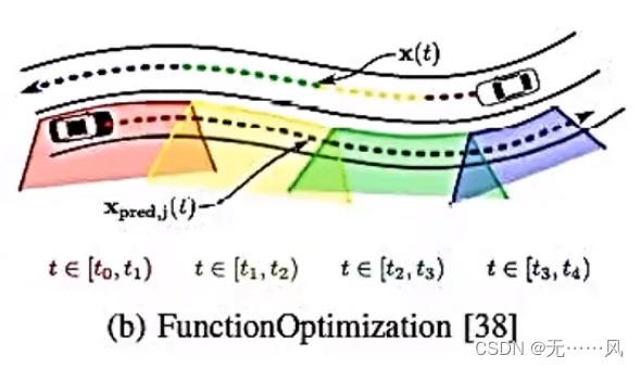
2. fuction optimization based on optimization
   

3. Sampling-based approach
   
   
   

4. Other methods (property types)

2. Nature of action planning (planner)

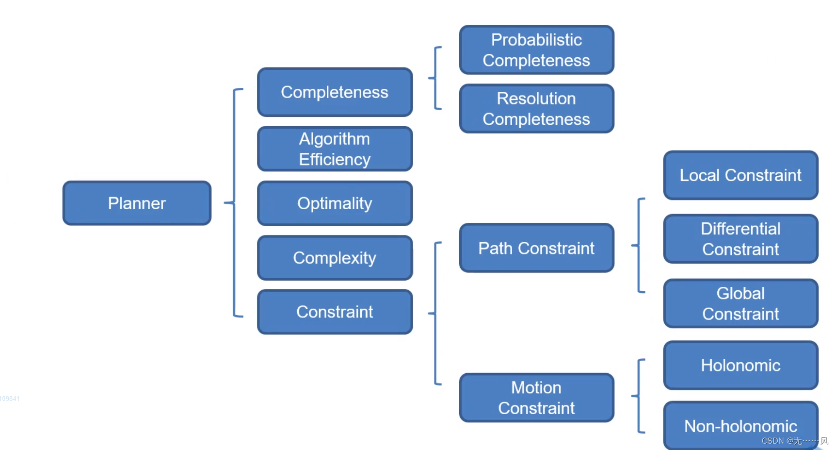
1. Completeness
   refers to whether a path can be found from the starting point to the end point, including probability completeness and decision-making completeness.
2. Alogrithm Efficiency
3. Optimality
4. Complexity (Solving Complexity Problems)
5. Constrain (performance under constraints)
   (1) Path constraints
   (2) Motion constraints

2.1 Completeness

1. Completeness: It means that if there is a path between the starting point and the target point, then an optimal solution will definitely be obtained. If it cannot be obtained, the solution does not exist, such as Narrow Gap Problem Examples. The narrow road cannot be passed.
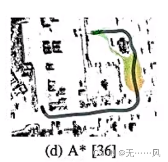
2. Complete planner: Within a certain period of time, the planner can always find a path from the starting point to the end point, such as the A* algorithm.
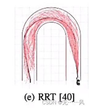
3. Probabilistic Completeness: There is a path between the starting point and the target point. If the planning and search time is long enough, you can use the sampling method to ensure that there is a solution to find this path, such as RRT and BIT* algorithms.
4. Decision Completeness (Resolution Completeness): The principle is very similar to that of probability completeness, but its sampling is relatively deterministic, usually on a grid.

2.2 Alogrithmic efficiency

Usually, the most important evaluation index of an algorithm is execution time. Although algorithm analysis also needs to consider the memory space required for operation, with the development of technology, space is no longer a factor to consider, so time complexity is first needed:

1. Time complexity representation (linear):
   
   usually represented by O.
2. The execution time of the algorithm is directly proportional to the amount of input data.

2.3 Optimality

1. The planned path is optimal on a certain evaluation index;
2. If there is no optimal one, consider asymptotic optimality. The suboptimal path that is close to the optimal one obtained in a limited number of planning iterations will gradually converge, and each iteration will be close to the optimal path.

2.4 Complexity

1. Space dimensionality (dimensional space)
   is a three-dimensional space for rigid bodies. For non-rigid bodies (large trailers and bicycle models), it is inaccurate to use a three-dimensional model.
2. How do Geometric complexity
   objects intersect;
   polygons and polygon trajectory exploration.

2.5 Path constraints

1. Local Constraints (local constraints)
   avoid collisions with obstacles;
2. Differential contrains
   limit the vehicle’s path curvature and steering wheel angle;
3. Global constarins
   find the shortest path.

2.6 Holonomic vs non-holonomic constraint

Integrity constraints: the controllable degrees of freedom are equal to the total degrees of freedom;
non-integrity constraints: the controllable degrees of freedom are less than the total degrees of freedom;

3. Path planning

The essence of motion planning: searching for a good path.

3.1 where to search

So how to search for a good path? When starting research, humans often start with a particle model to study, but it turns into two points. Mathematically, there is no intersection between points and there is no way to collide. In fact, vehicles may collide with each other. Therefore, it is actually necessary to abstract a vehicle model to solve the problem of collision between vehicles and obstacles.

configuration space

In order to solve the above problems, the concept of constructed space is proposed, which is the tool for its processing.

1. Robotics: Consider practical physical constraints and rigid body dynamics issues;
2. Control theory: focus on stability and feedback, and consideration of future trends (the future speed space may collide in the future);
3. Artificial intelligence: consider logic and execution actions, change from initial state to desired state, Belief Space (belief space), Markov decision-making process, etc.

3.2 How to search

Combinatorial methods

It is a set of precise and complete solutions, such as the visibility graph,

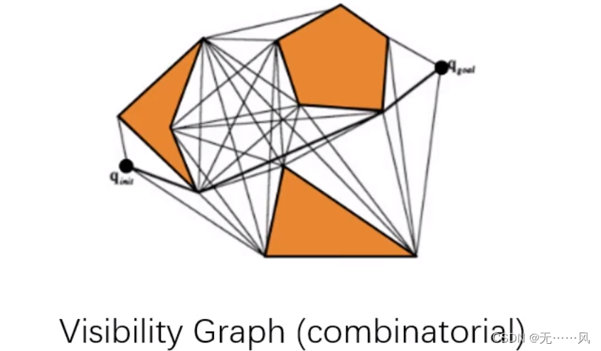
which is a road map constructed by connecting all nodes such as the starting point and the end point.
Node: includes the initial starting point, end point, and the vertices of all obstacles. Connect all points that do not intersect with obstacles, including the edges of obstacles. After establishing a visual chart, you can use the search algorithm to find the shortest path from the start to the end point. path.
**Disadvantages:** The search path often follows obstacles without leaving any space, which increases the risk of collision.

Sampling-based methods

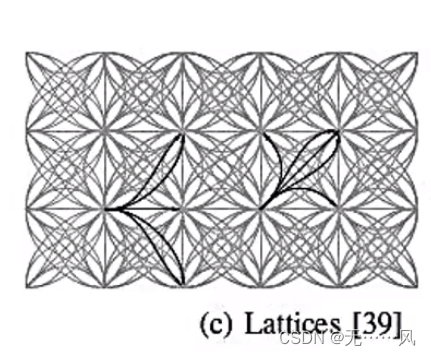
1. The determined sampling points (decision completeness)
   include grids and road structure maps.
2. Random sampling (probabilistic completeness)
   includes random sampling methods that require smoothing and post-processing to improve the quality of route construction.

3.3 Stochastic Sampling Methods

Traditional path planning algorithms: artificial potential field method, genetic algorithm, neural network, ant colony optimization algorithm, etc. all need to model obstacles in a determined space, and the computational complexity is exponentially related to the robot's degree of freedom. Suitable for solving complex planning problems in multi-degree-of-freedom environments.

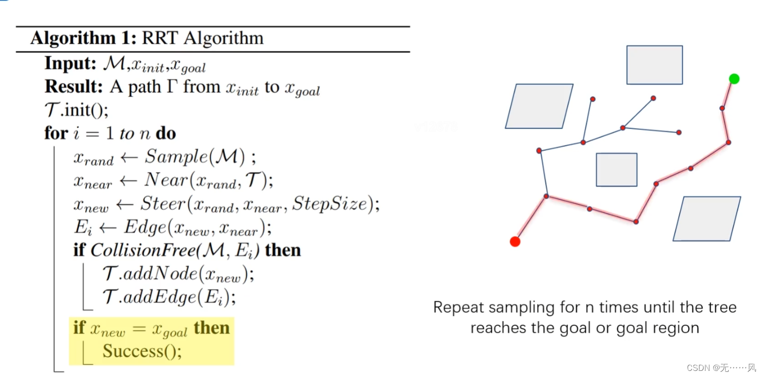
RRT

The RRT-based planning algorithm detects collisions through sampling points in the state space, avoiding modeling of the space, and can effectively solve high-dimensional planning space and complex constraint planning problems.
Features of RRT:
(1) Quickly and effectively search high-dimensional space, and guide the search to a blank area through random sampling points in the state space, thereby finding a planned path from the starting point to the target point.
RRT applications:
(1) Suitable for solving dynamic programming problems in complex environments with multiple degrees of freedom.
RRT pseudo code:

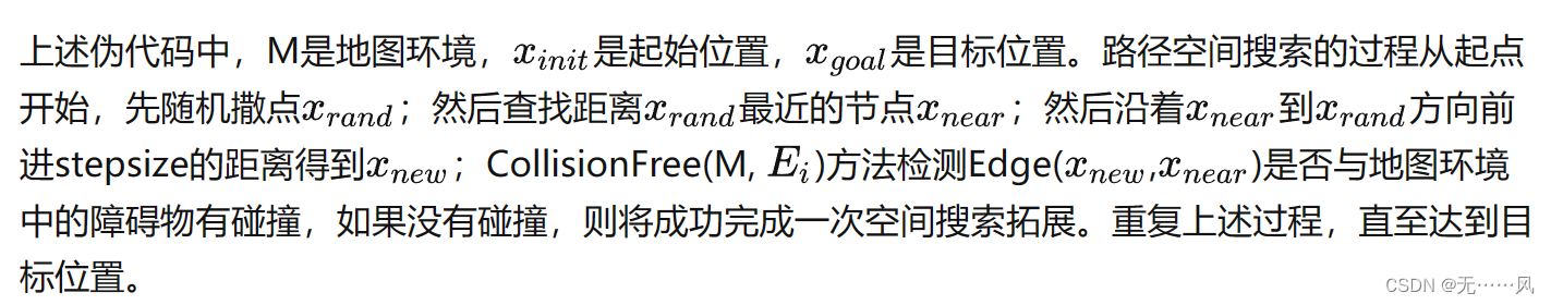
Advantages of RRT:
(1) Easy to implement and relatively intuitive;
(2) Find a path from the starting point to the target point;
(3) Target the unexplored part of the space.
Disadvantages of RRT:
(1) Not the optimal solution
(2) Not particularly efficient
(3) Sampling of the entire space

RRT*

Generally speaking, the RRT algorithm is a relatively efficient algorithm and can handle trajectory planning problems with non-holonomic constraints very well. It has great advantages in many aspects, but the RRT algorithm does not guarantee the feasibility of its results. The path is relatively optimized, so the RRT algorithm needs to be improved to solve the optimization problem. The RRT* algorithm is one of the optimization algorithms.

RRT features:
(1) The initial path can be quickly found, and as the sampling points continue to increase, optimization will continue until the target point is reached or the maximum number of cycles is reached; (2) Asymptotic optimization, as the number of iterations increases
, The obtained paths are becoming more and more optimized;
(3) The cost of RRT path generation is much smaller than that of RRT, which reduces the time cost.

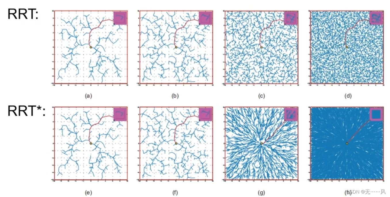
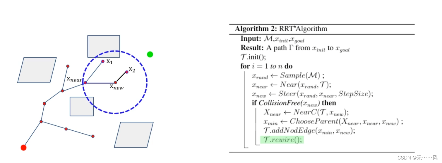
The difference between RRT* and RRT:
(1) Reselect the parent node (xnear): the path cost is relatively small;
(2) Rewiring: Reduce the redundancy of the random numbers after the new node.

3.4 Obstacle avoidance

In order to simplify the problem, relatively standard geometric shapes will be selected for path planning obstacles: circles, polygons, rectangles, etc.

circle object

The boundary of a circle is a nonlinear problem. The circle is usually linearized:
it only needs to be judged whether Xnew is within the square circumscribed by the circle. If it is, it means a collision.

polygon: rectangle (rectangular obstacle)

The sides of the line connecting Xnear and Xnew cannot intersect with any side of the rectangular obstacle.

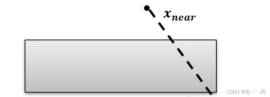
1. Xnear and Xnew are on one side of the rectangle and do not intersect with the matrix.
2. Xnear and Xnew are on different sides of one side of the rectangle:
   (1) Xnear and Xnew must intersect if they are inside the rectangle;
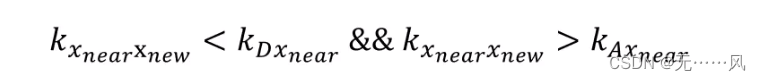
   (2) Xnear and Xnew are both outside the rectangle (solved by the slope method):
   
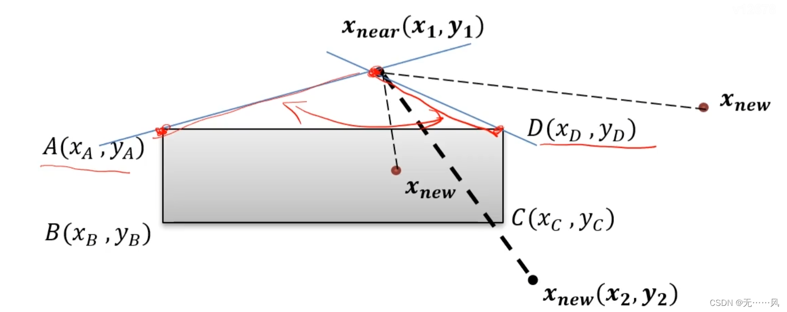
   If the following formula is satisfied, a collision will occur.
   

3.5 Other improvement methods

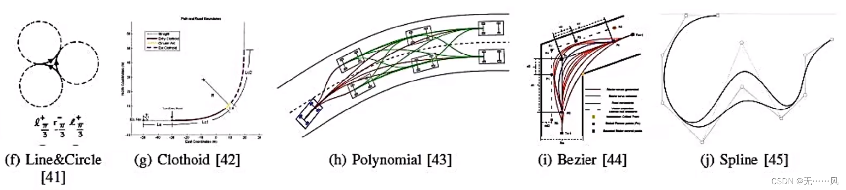
interpolation fitting

In practical applications, paths obtained using RRT or RRT* often have discontinuities, which affects the tracking difficulty and comfort of the vehicle.
Therefore, based on the existing Path point set and curvature, interpolation fitting is used to fit a drivable path, which has continuity and high derivability, and will improve vehicle tracking and comfort.
Interpolation fitting method:
3. Dubins
is the shortest path connecting two two-dimensional planes (x, y) when it satisfies the curvature constraint and the specified start-end and end-tangential direction conditions, and is only applicable to scenarios where the vehicle is moving forward.
4. Reeds-Shepp
is suitable for scenarios where the vehicle is moving backwards and forwards.
Due to the fixed geometry, Dubins and Reeds-Shepp can accurately calculate the distance between the vehicle and the path.
5. Spline, clothoid, and Bezier can improve the performance of interpolation fitting.

Solving efficiency

Core idea: Get closer to the target, guide the tree to a more open area, try to stay away from obstacles, and avoid repeated checks at obstacles to improve solution efficiency.

1. Bias Sampling
   makes the sampling points bias towards the target point as much as possible. During the random sampling process, the target state is inserted at a certain proportion to guide the tree to expand toward the target state, speed up the solution speed, and improve the solution quality.
   The standard RRT algorithm samples the space uniformly. If the target points are added to the uniform sampling points, the tree can be guided to move closer to the target faster.
2. Sample Rejection, Tree Pruning, and Graph Sparsify
   reject bad samples to increase the chance of sample success.
3. Delay Collision Check
   adds a penalty to the trajectory node and collision obstacle corresponding to each input. The higher the penalty, the smaller the probability of node expansion. It can limit the sampling area to the local area of ​​the current tree to prevent repeated expansion failures close to the target node to improve efficiency of the algorithm.
4. Anytime RRT
   quickly constructs RRT, obtains a record of feasible solutions, records its cost, and then performs sampling. In this way, the algorithm only inserts more trees in places that are beneficial to reducing the loss of feasible solutions, thereby obtaining better feasible solutions.

---

Summarize

This article mainly studies action planning in autonomous driving planning control. It mainly introduces the concept, properties and random sampling method of action planning, compares RRT and RRT*, and briefly talks about its improvement method. This article hopes to be of some help to students who want to learn the direction of autonomous driving planning and control.
Friends who like it, move your little hands and click on it. I will regularly share some of my knowledge summaries and experiences. Thank you all!