4. Planning control - optimal control of vehicle trajectory tracking (2)

Overview: This article mainly studies the optimal control of vehicle trajectory tracking - LQR

---

foreword

This paper will continue to study the optimal control of trajectory tracking of autonomous driving vehicles-LQR.

---

Linear quadratic regulator (LQR, Linear quadratic regulator)

LQR concept:

1. principle

The system assigns a cost to each path from state A to state B, and selects the optimal solution of the smallest path. The process of determining the optimal solution is to design the weight of each cost. Extending its thinking to the control system, then the process of optimizing this controller is the process of choosing what (system performance, cost, etc.) is more important to us.

2. Research object
   The research object of LQR is based on the linear system given by the state space model.
   

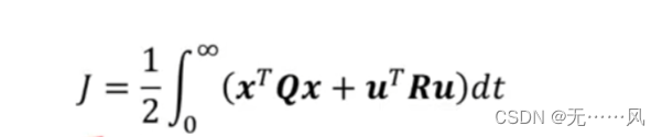
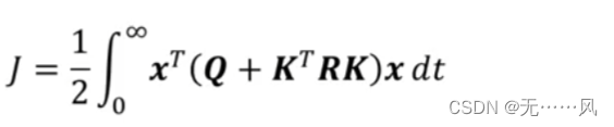
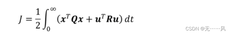
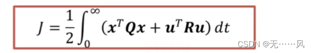
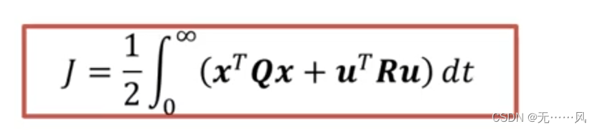
3. Objective function (loss function)
   LQR objective function is a quadratic function of object state and control input.
   
   (1) The integral area of ​​the quadratic function is positive, which more accurately shows the speed of the response regression; (
   2) The quadratic function is a convex function, and there must be a local minimum, so that the loss function can be guaranteed to have a The minimum value;
   (3) The penalty will be accelerated after the quadratic function is squared.

4. The task of the task
   LQR is to return the state and input of the system to the equilibrium state without consuming excess energy when the state of the system deviates from the equilibrium state for any reason. Generally speaking, 0 is regarded as the equilibrium state.

Generally, the area of ​​the response is used to replace the size of the cost. When the area is smaller, the cost is smaller and can return to the equilibrium state faster.

Therefore, the purpose of LQR is to adjust all states and inputs of the system whose initial state is not 0 to 0, and minimize the cost function.

Objective function analysis

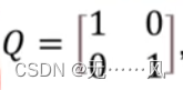
Among them, Q and R refer to the ratio between the state and the input weight. Generally speaking, the Q and R matrices can be written in the form of a diagonal matrix: the elements on the diagonal matrix



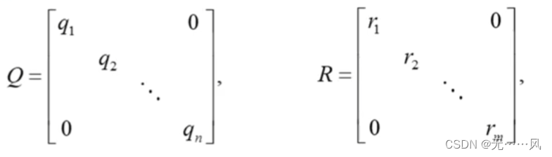
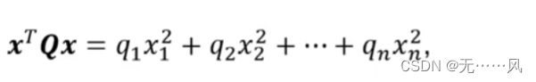
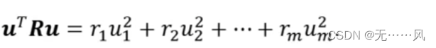
represent the weight of the state quantity and the control quantity, The greater the weight, the greater the importance attached to the quantity, and the greater the penalty for this quantity. If the importance of each quantity is the same, the diagonal matrix can be taken as an identity matrix.

LQR parsing based on 1D scalar systems (a scalar example)

Assume a system with as few control inputs as possible and as close to 0 as possible during regression:

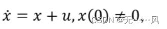
where both A and B are equal to 1 and the initial state is not 0.

Therefore, the objective function J should be as small as possible:

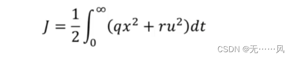
where, q>=0, the state error measure is positive; r>0, the control input error measure is positive.

To make the objective function as small as possible, the following steps are required:

1. Assuming that
   
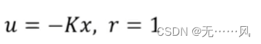
   among them, let r be 1, you only need to adjust the ratio of q.

2. Bring the above formula into the system and objective function:

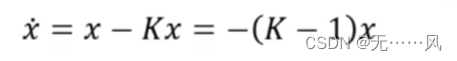
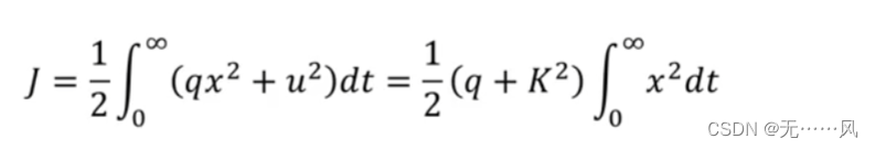
3. Solving linear differential equations:
   
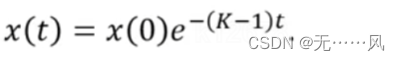
   When k>1, the function converges and the system is stable.

4. Bring x(t) back to the objective function:

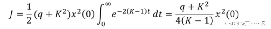
5. Under the condition of fixing q and x(0), to find the minimum value of the objective function, it is necessary to find that the first-order partial derivative of K is equal to 0, and the second-order partial derivative is greater than or equal to 0.

Then the first order derivative of the objective function:

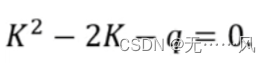
Finding the second partial derivative:

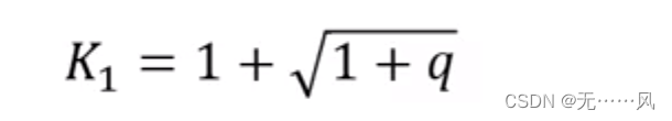
Then: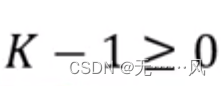
Since K>=1, q>=0, in the solution of K obtained above, only K1 satisfies the condition, which verifies the requirement of K value for system stability.

Then the minimum value of the objective function is:

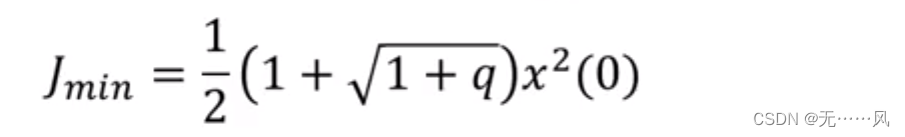
In summary,
the system problem is transformed into adjusting the value of q. When the value of q is larger, the value of K is larger, and the speed of the state response (close to 0) is accelerated. At this time, the most important thing is to correct the error ; When the value of q is small, it is equivalent to indirectly increasing the weight r of the control input. At this time, more attention is paid to the consumption (quantity) of the input.

LQR analysis (raccati equation) based on n-dimensional system

Assume a system:

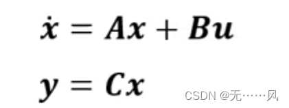
where x is an n×n-dimensional matrix, and u is an n-dimensional matrix.

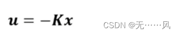
1. Assume that there is a value of K such that the system is stable.

2. Bring the above formula into the system and objective function
   
   

3. Introduce the P matrix, an N×N symmetric matrix, so that x and u eventually approach 0.
   

4. The above formula can be brought into the objective function
   
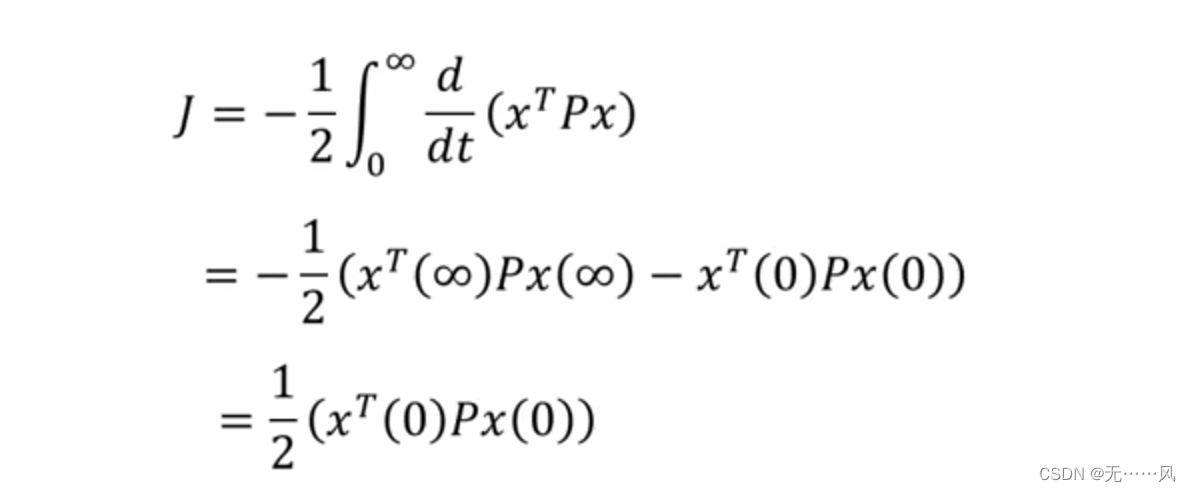
   , so that the process of solving the objective function J can be transformed into the process of solving P.
   

(1) Since the K term is unknown, remove the K term and expand the above equation first:

(2) Bring the system function into the above formula:


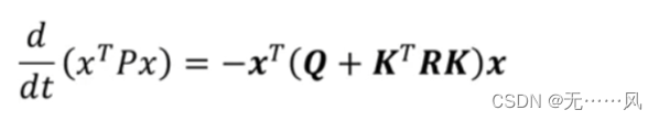
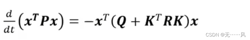
(3) For the quadratic function equal to 0, the middle term must be 0 .

(4) The system function reverses back to the above formula:

(5) Let K be the following formula:


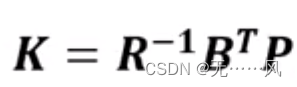
(6) Riccati equation (algebraic Riccati equation, CARE)

where A and B are known, and Q can be adjusted. Only P is unknown, P can be obtained, and then the objective function can be obtained.

Summary:
For linear systems,

there is always such a control rate:

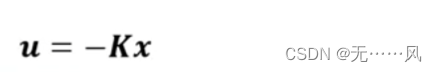
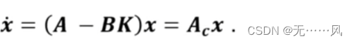
Make closed-loop systems:

Minimize the loss function:

Introduce P to make the system close to 0:

get P by raccati equation:

LQR tuning

Q fixed

1. Assuming Q is fixed:

2. Choose different R:
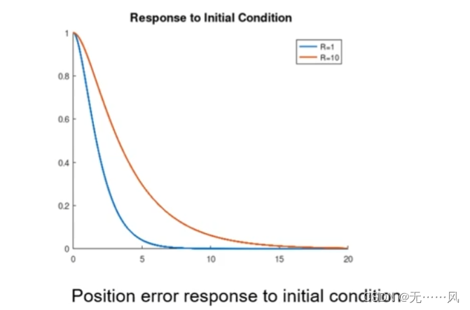
   (1) When R is selected as 10, the influence on the input u will be greater, and the influence on the state x will be smaller, and the control amount will be used less, so that the control input regression response will be faster, making the system The regression response (position error regression response) becomes slower.
   (2) When R selects 1, the influence on the input u will be smaller, and the influence on the state x will be greater, and more control variables will be used, which will slow down the regression response of the control input and make the system regression response (position error Regression response) becomes faster.

fixed

1. Assuming R is fixed:
   
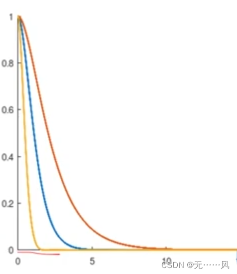
2. Choose a different Q:
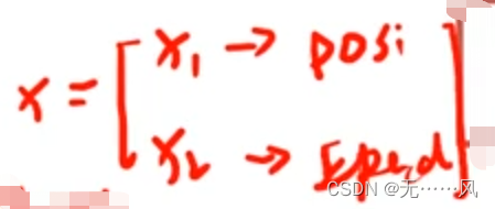
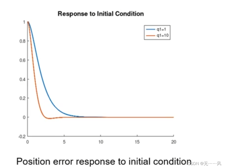
   Since Q is related to the adjustment of the state quantity, at this time x1 is the position and x2 is the speed:
   

(1)
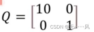
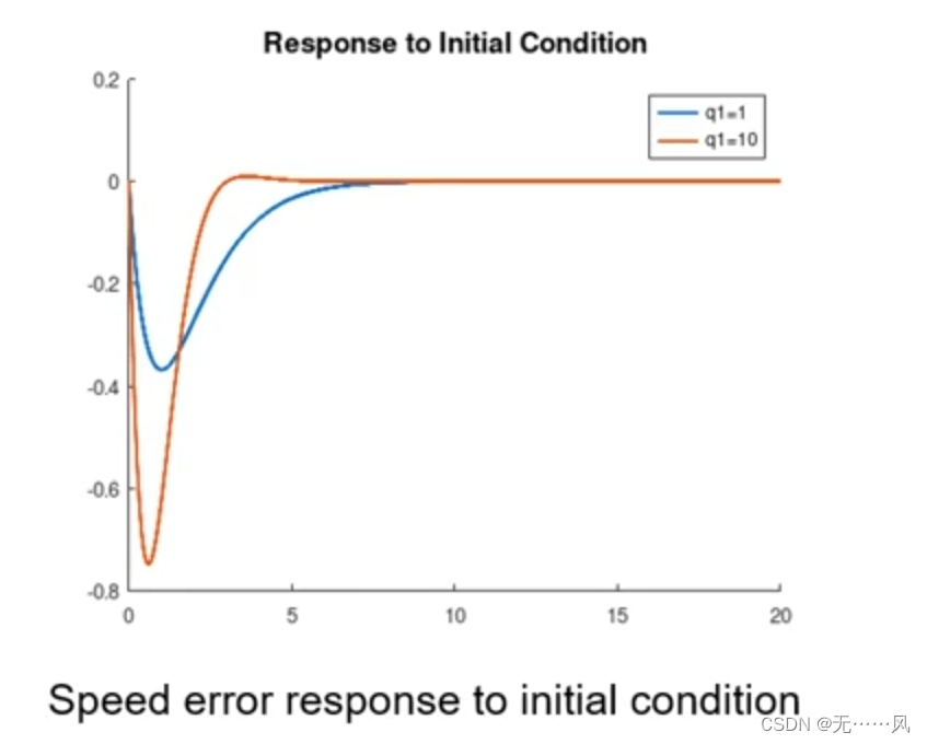
When q1=10 and q2=1 are selected, the penalty on the position error has the greatest influence, and the penalty on the speed has the least influence, but the overall penalty is greater than the input, and the system will have a fast regression response, but it needs to be Input takes more effort to achieve this quick response.

(2)
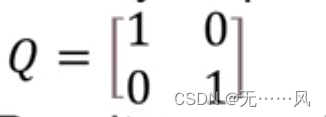
When q1=1 and q2=1, the penalty effect on the position error is equal to the penalty effect on the speed, and the regression response of the system is relatively slow, but the energy consumption of the control input is relatively small.

In general, LQR adjustment is the proportional adjustment of Q and R, focusing on the relative proportional relationship between Q and R, that is, the increase of Q has the same effect as the decrease of R, and the proportion and weight will not change.
LQR adjustment depends on the situation:
(1) When choosing a faster system response and not caring about the control input, you can make the Q adjustment larger and optimize Q first.
(2) When you are very concerned about the control input (energy consumption of the controller), you can adjust R to be larger, and optimize R first.

---

Summarize

This article is mainly for the learning of optimal control of trajectory tracking in automatic driving planning control. It mainly introduces the concept, analysis and adjustment of LQR. This article hopes to have a certain understanding for students who want to learn the direction of automatic driving planning control help.
Friends who like it, move your little hands to follow, I will regularly share some of my knowledge summaries and experiences, thank you!