Table of contents

Example 2

1.2 Multivariate

Example 3

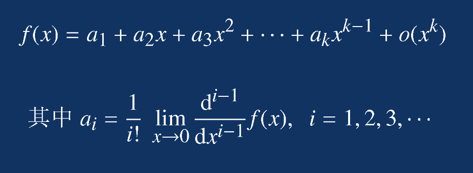
2. Fourier series expansion

1. Taylor power series expansion

1.1 Univariate

The Taylor power series around the point x=0 is as follows:

Expand at x=a:

MATLAB format:

%x=0进行Taylor幂级数展开
taylor(f,x,k)

%x=a进行Taylor幂级数展开
taylor(f,x,k,a)

Example 1

Find the first 9 terms of the Taylor power series expansion of the function; and find the Taylor power series expansion for x=2 and x=a.

$f(x)=\frac{sinx}{x^2+4x+3}$

untie:

MATLAB code:

clc;clear;
syms x a;
f=sin(x)/(x^2+4*x+3);
y1=taylor(f,x,'order',9);
pretty(y1)

taylor(f,x,2,'order',9)

taylor(f,x,a,'order',5)

operation result:

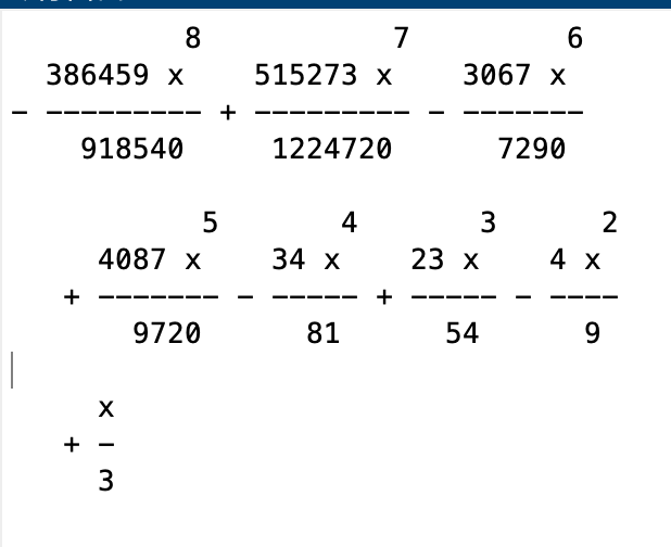
ans =sin(2)/15 - ((131623*cos(2))/35880468750 + (875225059*sin(2))/34445250000000)*(x - 2)^8 + (x - 2)*(cos(2)/15 - (8*sin(2))/225) - ((623*cos(2))/11390625 + (585671*sin(2))/2733750000)*(x - 2)^6 + ((262453*cos(2))/19136250000 + (397361*sin(2))/5125781250)*(x - 2)^7 - (x - 2)^2*((8*cos(2))/225 + (127*sin(2))/6750) + (x - 2)^3*((23*cos(2))/6750 + (628*sin(2))/50625) + (x - 2)^4*((28*cos(2))/50625 - (15697*sin(2))/6075000) + (x - 2)^5*((203*cos(2))/6075000 + (6277*sin(2))/11390625)

ans =sin(a)/(a^2 + 4*a + 3) - (cos(a)/(a^2 + 4*a + 3) - (sin(a)*(2*a + 4))/(a^2 + 4*a + 3)^2)*(a - x) - (a - x)^2*(sin(a)/(2*(a^2 + 4*a + 3)) + (cos(a)*(2*a + 4))/(a^2 + 4*a + 3)^2 - (sin(a)*((2*a + 4)^2/(a^2 + 4*a + 3)^2 - 1/(a^2 + 4*a + 3)))/(a^2 + 4*a + 3)) - (a - x)^3*((sin(a)*((2*a + 4)/(a^2 + 4*a + 3)^2 - (((2*a + 4)^2/(a^2 + 4*a + 3)^2 - 1/(a^2 + 4*a + 3))*(2*a + 4))/(a^2 + 4*a + 3)))/(a^2 + 4*a + 3) - cos(a)/(6*(a^2 + 4*a + 3)) + (cos(a)*((2*a + 4)^2/(a^2 + 4*a + 3)^2 - 1/(a^2 + 4*a + 3)))/(a^2 + 4*a + 3) + (sin(a)*(2*a + 4))/(2*(a^2 + 4*a + 3)^2)) + (a - x)^4*(sin(a)/(24*(a^2 + 4*a + 3)) - (sin(a)*(((2*a + 4)^2/(a^2 + 4*a + 3)^2 - 1/(a^2 + 4*a + 3))/(a^2 + 4*a + 3) + ((2*a + 4)*((2*a + 4)/(a^2 + 4*a + 3)^2 - (((2*a + 4)^2/(a^2 + 4*a + 3)^2 - 1/(a^2 + 4*a + 3))*(2*a + 4))/(a^2 + 4*a + 3)))/(a^2 + 4*a + 3)))/(a^2 + 4*a + 3) + (cos(a)*((2*a + 4)/(a^2 + 4*a + 3)^2 - (((2*a + 4)^2/(a^2 + 4*a + 3)^2 - 1/(a^2 + 4*a + 3))*(2*a + 4))/(a^2 + 4*a + 3)))/(a^2 + 4*a + 3) + (cos(a)*(2*a + 4))/(6*(a^2 + 4*a + 3)^2) - (sin(a)*((2*a + 4)^2/(a^2 + 4*a + 3)^2 - 1/(a^2 + 4*a + 3)))/(2*(a^2 + 4*a + 3)))

Example 2

Perform Taylor power series expansion on sinx, and observe the approximation effect of different orders.

untie:

MATLAB code:

clc;clear;
x0=-2*pi:0.01:2*pi;
y0=sin(x0);
syms x;
y=sin(x);
plot(x0,y0,'r-'),axis([-2*pi,2*pi,-1.5,1.5]);
hold on 
for n=[8:2:16]
    p=taylor(y,x,'order',n),
    y1=subs(p,x,x0);
    line(x0,y1);
end

operation result:

p =- x^7/5040 + x^5/120 - x^3/6 + x

p =x^9/362880 - x^7/5040 + x^5/120 - x^3/6 + x

p =- x^11/39916800 + x^9/362880 - x^7/5040 + x^5/120 - x^3/6 + x

p =x^13/6227020800 - x^11/39916800 + x^9/362880 - x^7/5040 + x^5/120 - x^3/6 + x

p =- x^15/1307674368000 + x^13/6227020800 - x^11/39916800 + x^9/362880 - x^7/5040 + x^5/120 - x^3/6 + x

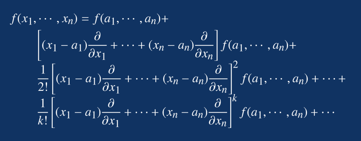
1.2 Multivariate

The Taylor power series expansion of the multivariate function $f(x_1,x_2,\cdots,x_n)$ in is as follows: $(a_1,a_2,\cdots,a_n)$

Example 3

Find various Taylor power series expansions of z=f(x,y).

$z=f(x,y)=(x^2-2x)e^{-x^2-y^2-xy}$

untie:

MATLAB code:

clc;clear;
syms x y a;
f=(x^2-2*x)*exp(-x^2-y^2-x*y);
F1=taylor(f,[x,y],[0,0],'order',8)
F2=taylor(f,[x,y],[1,a],'order',3)

operation result:

F1 =
x^7/3 + x^6*y + x^6/2 + 2*x^5*y^2 + x^5*y - x^5 + (7*x^4*y^3 )/3 + (3*x^4*y^2)/2 - 2*x^4*y - x^4 + 2*x^3*y^4 + x^3*y^3 - 3* x^3*y^2 - x^3*y + 2*x^3 + x^2*y^5 + (x^2*y^4)/2 - 2*x^2*y^3 - x^2*y^2 + 2*x^2*y + x^2 + (x*y^6)/3 - x*y^4 + 2*x*y^2 - 2*x F2

=
( exp(- a^2 - a - 1) - exp(- a^2 - a - 1)*((a/2 + 1)*(a + 2) - 1))*(x - 1)^2 - exp(- a^2 - a - 1) - exp(- a^2 - a - 1)*(a - y)^2*((2*a + 1)*(a + 1/2) - 1) + exp(- a^2 - a - 1)*(a + 2)*(x - 1) - exp(- a^2 - a - 1)*(2*a + 1)*(a - y) + exp(- a^2 - a - 1)*(a - y)*(x - 1)*((2*a + 1)*(a/2 + 1) + (a + 2)* (a + 1/2) - 1)

2. Fourier series expansion

Given f(x) and the following conditions:

$x\in[-L,L],T=2L,f(t)=f(kT+t)$

Fourier series, as follows:

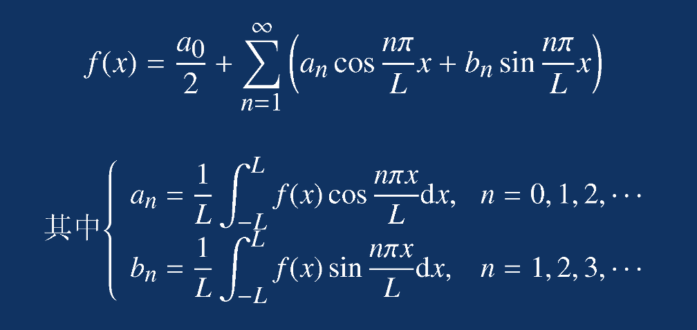
Write an analytic function for Fourier series:

function [A,B,F]=fseries(f,x,n,a,b)
if nargin==3,a=-pi;
    b=pi;
end
L=(b-a)/2;
if a+b, f=subs(f,x,x-L-a);
end %变量区域互换
A=int(f,x,-L,L)/L;
B=[];
F=A/2; %计算a0
for i=1:n
    an=int(f*cos(i*pi*x/L),x,-L,L)/L;
    bn=int(f*cos(i*pi*x/L),x,-L,L)/L;
    A=[A,an];
    B=[B,bn];
    F=F+an*cos(i*pi*x/L)+bn*sin(i*pi*x/L);
end
if a+b,
    F=subs(F,x,x+L+a);
end %换回变量区域
end

Example 4

Find the Fourier series expansion of y.

$y=x(x-\pi)(x-2\pi),\quad x\in(0,2\pi)$

untie:

MATLAB code:

clc;clear;
syms x;
f=x*(x-pi)*(x-2*pi);
[A,B,F]=fseries(f,x,6,0,2*pi)


function [A,B,F]=fseries(f,x,n,a,b)
if nargin==3,a=-pi;
    b=pi;
end
L=(b-a)/2;
if a+b, f=subs(f,x,x-L-a);
end %变量区域互换
A=int(f,x,-L,L)/L;
B=[];
F=A/2; %计算a0
for i=1:n
    an=int(f*cos(i*pi*x/L),x,-L,L)/L;
    bn=int(f*sin(i*pi*x/L),x,-L,L)/L;
    A=[A,an];
    B=[B,bn];
    F=F+an*cos(i*pi*x/L)+bn*sin(i*pi*x/L);
end
if a+b,
    F=subs(F,x,x+L+a);
end %换回变量区域
end

operation result:

A =[ -16*ft^3, 24*ft, -6*ft, (8*ft)/3, -(3*ft)/2, (24*ft)/25, -(2*ft) /3]

B =
[ -(12*ft - 24*ft^3)/ft, ((3*ft)/2 - 12*ft^3)/ft, -((4*ft)/9 - 8 *ft^3)/ft, ((3*ft)/16 - 6*ft^3)/ft, (24*ft^2)/5 - 12/125, (ft/18 - 4*ft^3 )/pi]

F =
(sin(x)*(12*pi - 24*pi^3))/pi - 24*pi*cos(x) - 8*pi^3 - 6*pi*cos(2* x) - (8*pi*cos(3*x))/3 - (3*pi*cos(4*x))/2 - (24*pi*cos(5*x))/25 - (2 *pi*cos(6*x))/3 - sin(5*x)*((24*pi^2)/5 - 12/125) + (sin(2*x)*((3*pi) /2 - 12*pi^3))/pi + (sin(3*x)*((4*pi)/9 - 8*pi^3))/pi + (sin(4*x)*(( 3*pi)/16 - 6*pi^3))/pi + (sin(6*x)*(pi/18 - 4*pi^3))/pi

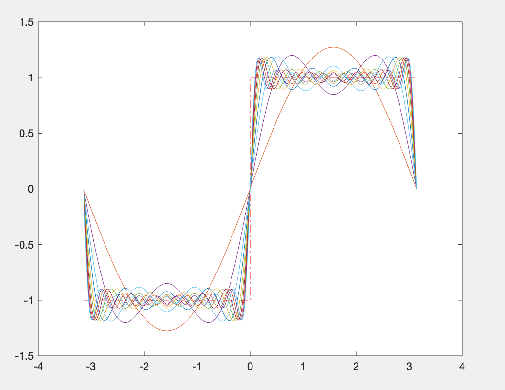
Example 5

For $(-\pee)$ the square wave signal in the interval, $x\geq 0$ at that time , y=1, otherwise y=-1. Carry out Fourier series fitting on it, and observe how many terms can have a better fitting effect.

untie:

MATLAB code:

clc;clear;
syms x;
f=abs(x)/x; %定义方波信号
xx=[-pi:pi/200:pi];
xx=xx(xx~=0);
xx=sort([xx,-eps,eps]); %剔除零点
yy=subs(f,x,xx);
plot(xx,yy,'r-.'), %绘制出理论值
hold on  %保持坐标系

for n=2:20
    [a,b,f1]=fseries(f,x,n);
    y1=subs(f1,x,xx);
    plot(xx,y1)
end


function [A,B,F]=fseries(f,x,n,a,b)
if nargin==3,a=-pi;
    b=pi;
end
L=(b-a)/2;
if a+b, f=subs(f,x,x-L-a);
end %变量区域互换
A=int(f,x,-L,L)/L;
B=[];
F=A/2; %计算a0
for i=1:n
    an=int(f*cos(i*pi*x/L),x,-L,L)/L;
    bn=int(f*sin(i*pi*x/L),x,-L,L)/L;
    A=[A,an];
    B=[B,bn];
    F=F+an*cos(i*pi*x/L)+bn*sin(i*pi*x/L);
end
if a+b,
    F=subs(F,x,x+L+a);
end %换回变量区域
end

operation result:

3. Series summation

given:

$S=\sum_{k=k_0}^{k_n}f_k$

Available in the Symbol Toolbox:

S=symsum(fk,k,k0,kn)

Example 6

Calculate the sum:

$S=2^0+2^1+2^2+2^3+2^4+\cdots+2^{62}+2^{63}=\sum_{i=0}^{63}2^i$

untie:

MATLAB code:

clc;clear;
format long;

%数值计算
sum(2.^[0:63])

%把2定义为符号量，计算会更准确
sum(sym(2).^[0:63])

%工具箱
syms k;
symsum(2^k,0,63)

operation result:

ans =1.844674407370955e+19

years =18446744073709551615

years =18446744073709551615

Example 7

Try to find the sum of infinite series

$S=\frac{1}{1\times 4}+\frac{1}{4\times 7}+\frac{1}{7\times 10}+\cdots+\frac{1}{(3n-2)\times (3n+1)}+\cdots$

untie:

MATLAB code:

clc;clear;

%符号工具箱
syms n;
s=symsum(1/((3*n-2)*(3*n+1)),n,1,inf)

%数值计算
format long %以长型方式显示得出的结果
m=1:1000000;
s1=sum(1./((3*m-2).*(3*m+1))) %双精度有效位16

operation result:

s =1/3

s1 =0.333333222222265

Example 8

Solve:

$J=2\sum_{n=0}^\infty\frac{1}{(2n+1)(2x+1)^{2n+1}}$

untie:

MATLAB code:

clc;clear;
syms n x;
s1=symsum(2/((2*n+1)*(2*x+1)^(2*n+1)),n,0,inf)

operation result:

s1 =piecewise(1 < abs(2*x + 1), 2*atanh(1/(2*x + 1)))

Example 9

beg:

$\lim_{n\to\infty}[(1+\frac{1}{2}+\frac{1}{3}+\frac{1}{4}+\cdots++\frac{1}{n})-lnn]$

untie:

MATLAB code:

clc;clear;
syms m n;
limit(symsum(1/m,m,1,n)-log(n),n,inf);
vpa(ans,70)  %显示70位有效数字

operation result:

ans =

0.5772156649015328606065120900824024310421593359399235988057672348848677

Power series summation and expansion based on MATLAB (Taylor and Fourier algorithm)

1. Taylor power series expansion

1.1 Univariate

Example 1

Example 2

1.2 Multivariate

Example 3

2. Fourier series expansion

Example 4

Example 5

3. Series summation

Example 6

Example 7

Example 8

Example 9

Guess you like