Large language models have been used in many fields, and their applications include intelligent writing, music creation, knowledge quiz, chat, customer service, advertising copywriting, papers, news, novel writing, polishing, conference/article summaries, etc. In business, the model is the product, the service is the product, and the plug-in is the product. Any form of user-accessible products can be products. Commercial payments are generally membership-based or pay-per-use. The core structure of the current big prophecy model is based on Transformer.
A very important reason why the effect of the large model exceeds expectations is that the model will undergo qualitative changes after it reaches a certain level, and the memory and generalization of the model can be combined. Transformer can make the model very large, so large that the model in the NLP field can undergo qualitative changes, which allows applications to appear in various fields, but there are still some problems that need to be further solved. This type of large model is essentially content generation. The content conforms to the following three principles:
helpful (Helpful);
credible (Honest);
harmless (Harmless)
The big prediction model (also known as the pretraining model) based on the Transformer framework alone is not enough to fully meet the requirements of commercial applications. The development of the industry will be unfolded in a follow-up blog. This article will first talk about Transformer, the core architecture of the big language model.
Transformer originated from Google Brain's proposal for machine translation tasks in 2017. The paper "Attention is all you need" explained the network structure in detail. Before this, the network structure mostly used RNN, CNN, LSTM, GRU and other network forms. This article proposes A new core structure-Transformer is redesigned for the weakness of the RNN network in machine translation. In the modeling process of the traditional Encoder-Decoder architecture, the calculation process at the next moment will depend on the output at the previous moment. , and this inherent property restricts the traditional Encoder-Decoder model from being able to perform calculations in parallel.
The source code of this article has been hosted at the github link address
Model Structure Introduction
The Transformer proposed by Google also includes two parts: Encoder and decoder, but the core of these two parts is the Attention structure, not CNN, LSTM, GRU and other structures.
For the Encoder, it contains two layers, a self-attention layer and a feed-forward neural network. Self-attention can help the current node not only focus on the current word, but also obtain the semantics of the context. Decoder also includes the two-layer network mentioned by encoder, but there is an attention layer between the two layers to help the current node obtain the key content that needs to be paid attention to at present.
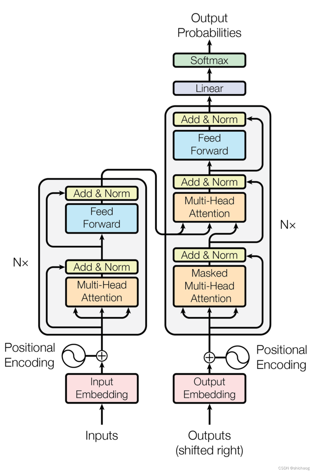
The Transformer model architecture
model needs to perform an embedding operation on the input data (the red box in the figure). Although Attention can extract the information of interest, it has no timing information, and Position Encoding is realized by converting timing information into position information. After the enmbedding is finished, the position code is added, and then input to the encoder layer. After the self-attention processes the data, the data is sent to the feed-forward neural network (blue Feed Forward). The calculation of the feed-forward neural network can be parallelized, and the output obtained will be Input to the next encoder.
- Encoder encoder
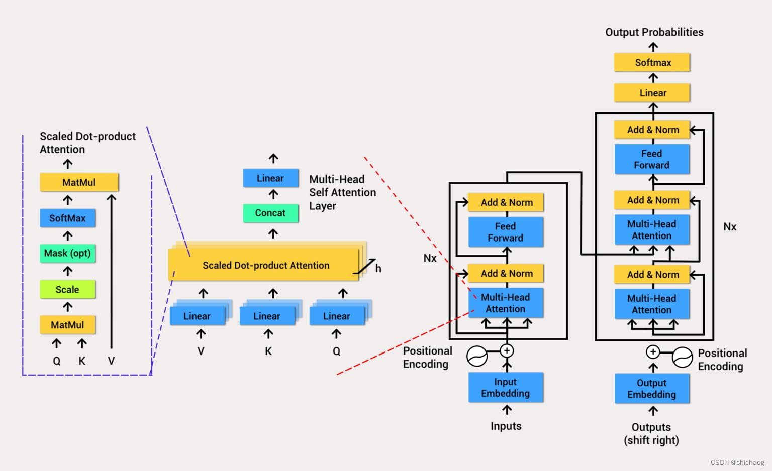
- Multi-Head Attention
- The multi-head self-attention mechanism can calculate the query-key-value (Query-Key-Value) in parallel by inputting information, so that the subsequent network can use the context to know which information needs to be paid attention to in the current operation. Note that the matrix for calculating QKV here is also part of the network parameters, and training can make the network's attention more effective and focused. Because the NLP field is causal in time series, the improved model uses a causal multi-head self-attention model.
- Add residual connection
- The main role of the main residual connection here is to use identity mapping to train deeper networks (input and output identity), multi-head attention and layer normalization, feedforward neural network and layer normalization, both parts use residual connections.
- Norm layer normalization
- The function of Layer Normalization is to normalize the neural network with the sample dimension as a layer, so as to speed up the training speed and accelerate the convergence. The new improvements put Layer Normalization in front instead of behind.
- Feed Forward Feedforward Neural Network
- After passing through the attention layer, the attention information extracted through the weighting mechanism is converted in the semantic space according to the attention information.
- Therefore, MLP reprojects the vector obtained by Multi-Head Attention into a larger space (in the paper, the space is enlarged by 4 times). In that large space, it is more convenient to extract the required information (using the Relu activation function), and finally Project back to the original space of the token vector.
- Multi-Head Attention
- Decoder
- Basically the same as the Encoder, the composition is divided into Masked Multi-Head Attention, Masked Encoder-Decoder Attention (this layer is the attention layer connecting the encoder and the decoder, and because GPT only uses the encoder, this layer is deleted. .) And the Feed Forward neural network, each of the three parts has a residual connection, followed by a Layer Normalization. The following describes the Decoder's Masked Self-Attention and Encoder-Decoder Attention two parts,
- Masked Multi-Head Attention
- There is a problem with the Self-Attention mechanism. The complete labeled data during the training process will be exposed to the Decoder. This is obviously wrong. We need to perform some processing on the input of the Decoder. This processing is called Mask, and the data is selectively exposed to the Decoder (in GPT, it is equivalent to covering all the data behind, which are sequentially generated by the network).
- Multi-Head Attention
- Add residual connection
- Norm layer normalization
- Feed Forward Feedforward Neural Network
- The linear layer and Softmax
pass through the encoder and decoder, and finally a layer of fully connected layers and SoftMax (the later improved large language model uses Gaussian Error Linear Units function). The linear layer is a simple fully connected neural network that projects the vectors produced by the decoder stack into a larger vector called the logits vector. A Softmax layer (Softmax is an activation function for multiclass classification problems) converts vectors into probabilities (all positive and sum to 1.0). The unit with the highest probability is selected and the word associated with it is generated as output for this time step.
Model Pytorch implementation
The red part is input&output embedding.
class Embedder(nn.Module):
    def __init__(self, vocab_size, d_model):
        super().__init__()
        self.embed = nn.Embedding(vocab_size, d_model)

    def forward(self, x):
        #[123, 0, 23, 5] -> [[..512..], [...512...], ...]
        return self.embed(x)
location code
As shown in the following code, its value will be added to the above embedding and then input to the codec module.
class PositionalEncoder(nn.Module):

 def __init__(self, d_model: int, max_seq_len: int = 80):
     super().__init__()
     self.d_model = d_model

     #Create constant positional encoding matrix
     pos_matrix = torch.zeros(max_seq_len, d_model)

     # for pos in range(max_seq_len):
     #     for i in range(0, d_model, 2):
     #         pe_matrix[pos, i] = math.sin(pos/1000**(2*i/d_model))
     #         pe_matrix[pos, i+1] = math.cos(pos/1000**(2*i/d_model))
     #
     # pos_matrix = pe_matrix.unsqueeze(0) # Add one dimension for batch size

     den = torch.exp(-torch.arange(0, d_model, 2) * math.log(1000) / d_model)
     pos = torch.arange(0, max_seq_len).reshape(max_seq_len, 1)
     pos_matrix[:, 1::2] = torch.cos(pos * den)
     pos_matrix[:, 0::2] = torch.sin(pos * den)
     pos_matrix = pos_matrix.unsqueeze(0)


     self.register_buffer('pe', pos_matrix) #Register as persistent buffer

 def forward(self, x):
     # x is a sentence after embedding with dim (batch, number of words, vector dimension)
     seq_len = x.size()[1]
     x = x + self.pe[:, :seq_len]
     return x
self-attention
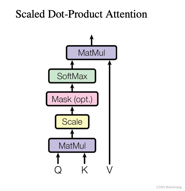
## Scaled Dot-Product Attention layer
def scaled_dot_product_attention(q, k, v, mask=None, dropout=None):
    # Shape of q and k are the same, both are (batch_size, seq_len, d_k)
    # Shape of v is (batch_size, seq_len, d_v)
    attention_scores = torch.matmul(q, k.transpose(-2, -1)) / math.sqrt(q.shape[-1]) # size (bath_size, seq_len, d_k)

    # Apply mask to scores
    # <pad>
    if mask is not None:
        attention_scores = attention_scores.masked_fill(mask == 0, value=-1e9)

    # Softmax along the last dimension
    attention_weights = F.softmax(attention_scores, dim=-1)

    if dropout is not None:
        attention_weights = dropout(attention_weights)

    output = torch.matmul(attention_weights, v)
    return output
Multi-Head Attention layer
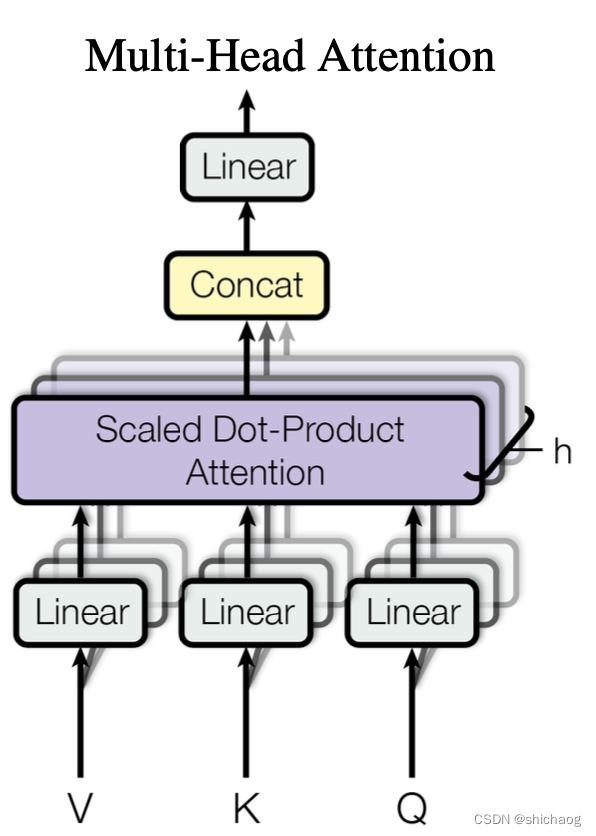
# Multi-Head Attention layer
class MultiHeadAttention(nn.Module):
    def __init__(self, n_heads, d_model, dropout=0.1):
        super().__init__()

        self.n_heads = n_heads
        self.d_model = d_model
        self.d_k = self.d_v = d_model // n_heads

        # self attention linear layers
        #Linear layers for q, k, v vectors generation in different heads
        self.q_linear_layers = []
        self.k_linear_layers = []
        self.v_linear_layers = []
        for i in range(n_heads):
            self.q_linear_layers.append(nn.Linear(d_model, self.d_k))
            self.k_linear_layers.append(nn.Linear(d_model, self.d_k))
            self.v_linear_layers.append(nn.Linear(d_model, self.d_v))

        self.dropout = nn.Dropout(dropout)
        self.out = nn.Linear(n_heads*self.d_v, d_model)

    def forward(self, q, k, v, mask=None):
        multi_head_attention_outputs = []
        for q_linear, k_linear, v_linear in zip(self.q_linear_layers,
                                                self.k_linear_layers,
                                                self.v_linear_layers):
            new_q = q_linear(q) # size: (batch_size, seq_len, d_k)
            new_k = q_linear(k) # size: (batch_size, seq_len, d_k)
            new_v = q_linear(v) # size: (batch_size, seq_len, d_v)

            # Scaled Dot-Product attention
            head_v = scaled_dot_product_attention(new_q, new_k, new_v, mask, self.dropout) # (batch_size, seq_len,
            multi_head_attention_outputs.append(head_v)

        # Concat
        # import pdb; pdb.set_trace()
        concat = torch.cat(multi_head_attention_outputs, -1) # (batch_size, seq_len, n_heads*d_v)

        # Linear layer to recover to original shap
        output = self.out(concat) # (batch_size, seq_len, d_model)

        return output
translation example
The github link here
shows the structure and usage of the network model described in Transformer's article with an English-to-French translation example. The Python installation version information is as follows:
Python 3.7.16
torch==2.0.1
torchdata==0.6.1
torchtext==0.15.2
spacy==3.6.0
numpy==1.25.2
pandas
times
portalocker==2.7.0
data processing
Tokenization and word mapping to tensorized numbers
It is more convenient to use the tools provided by torchtext to create a data set that is convenient for processing iterative speech translation models, starting with word segmentation from the original text, building a vocabulary, and marking it as a digital tensor. Although torchtext provides basic English word segmentation support, the translation here includes French in addition to English, so the word segmentation python library Spacy is used.
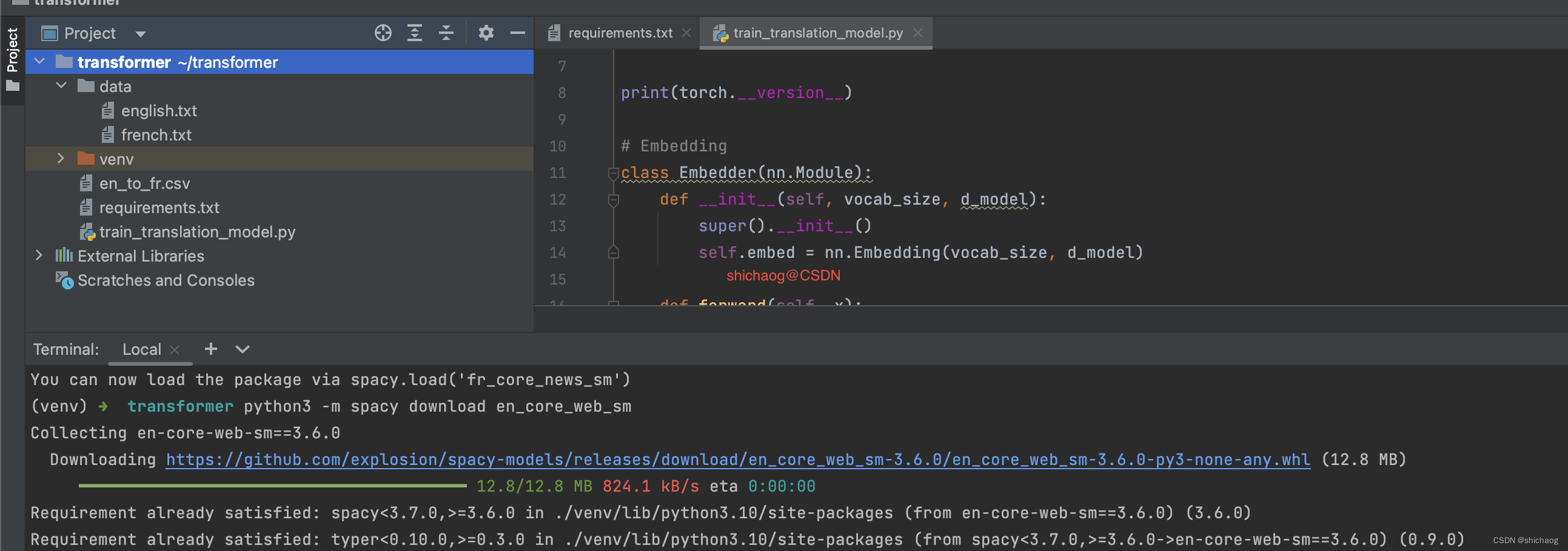
The first is to create the environment, and the next is to download the tokenizers for English and French, because this is a very small example, so use the spacy language processing model of the news:
#python3 -m spacy download en_core_web_sm
#python3 -m spacy download fr_core_news_sm
As shown below:
The next step is to segment the data into words, and then map the words into tensorized numbers
#Data processing
import spacy
from torchtext.data.utils import get_tokenizer
from collections import Counter
import io
from torchtext.vocab import vocab

src_data_path = 'data/english.txt'
trg_data_path = 'data/french.txt'

en_tokenizer = get_tokenizer('spacy', language='en_core_web_sm')
fr_tokenizer = get_tokenizer('spacy', language='fr_core_news_sm')


def build_vocab(filepath, tokenizer):
    counter = Counter()
    with io.open(filepath, encoding="utf8") as f:
        for string_ in f:
            counter.update(tokenizer(string_))
    return vocab(counter, specials=['<unk>', '<pad>', '<bos>', '<eos>'])

en_vocab = build_vocab(src_data_path, en_tokenizer)
fr_vocab = build_vocab(trg_data_path, fr_tokenizer)

def data_process(src_path, trg_path):
    raw_en_iter = iter(io.open(src_path, encoding="utf8"))
    raw_fr_iter = iter(io.open(trg_path, encoding="utf8"))
    data = []
    for (raw_en, raw_fr) in zip (raw_en_iter, raw_fr_iter):
        en_tensor_ = torch.tensor([en_vocab[token] for token in en_tokenizer(raw_en)], dtype=torch.long)
        fr_tensor_ = torch.tensor([fr_vocab[token] for token in fr_tokenizer(raw_fr)], dtype= torch.long)
        data.append((en_tensor_, fr_tensor_))
    return data

train_data = data_process(src_data_path, trg_data_path)
DataLoader
DataLoader is a method provided by torch.utils.data that combines datasets and samplers to provide iterable objects for a given dataset. DataLoader supports single-process or multi-process loading, custom load order and optional automatic batching (merging) and memory pinning of mapped and iterable datasets.
collate_fn (optional), which merges lists of samples to form mini-batches of tensors. Used when bulk loading with map-style datasets.
#Train transformer
d_model= 512
n_heads = 8
N = 6
src_vocab_size = len(en_vocab.vocab)
trg_vocab_size = len(fr_vocab.vocab)

BATH_SIZE = 32
PAD_IDX = en_vocab['<pad>']
BOS_IDX = en_vocab['<bos>']
EOS_IDX = en_vocab['<eos>']

from torch.nn.utils.rnn import pad_sequence
from torch.utils.data import DataLoader

def generate_batch(data_batch):
    en_batch, fr_batch = [], []
    for (en_item, fr_item) in data_batch:
        en_batch.append(torch.cat([torch.tensor([BOS_IDX]), en_item, torch.tensor([EOS_IDX])], dim=0))
        fr_batch.append(torch.cat([torch.tensor([BOS_IDX]), fr_item, torch.tensor([EOS_IDX])], dim=0))
    en_batch = pad_sequence(en_batch, padding_value=PAD_IDX)
    fr_batch = pad_sequence(fr_batch, padding_value=PAD_IDX)
    return en_batch, fr_batch

train_iter = DataLoader(train_data, batch_size=BATH_SIZE, shuffle=True, collate_fn=generate_batch)
The output of the training is as follows:
