2017 MathorCup Mathematical Modeling B Questions Shared Bicycle Problem Solving Process Documents and Programs

The 7th MathorCup University Mathematical Modeling Challenge in 2017

Question B Bike Sharing

Reproduction of the original title:

  Bike sharing refers to the bicycle sharing service provided by enterprises in campuses, subway stations, bus stations, residential areas, commercial areas, public service areas, etc., and is a time-sharing rental model. Bike sharing is a new type of sharing economy. Shared bicycles have attracted more and more people's attention, and because they conform to the concept of low-carbon travel, the government is also in a good-faith observation period for this new thing.
  The bicycles of many shared bicycle companies have GPS positioning, which can realize dynamic monitoring of vehicle data and riding distribution data, and then make all-weather supply and demand forecasts for bicycles, providing guidance for vehicle launch, dispatch, and operation and maintenance.
  Please complete the following questions according to the data given in the following attachment and combined with the data collected by yourself as needed:
  (1) According to the riding data of shared bicycles in Appendix 1, estimate the spatial and temporal distribution of shared bicycles. For example, starting from a certain point A, the distribution of arriving at different points. Discussion can be divided into time periods.
  (2) If the estimated data of people's cycling demand is obtained according to the survey, see Appendix 2.
  According to the estimated results of problem 1, a mathematical model is established to solve the problem of how to optimize the scheduling of shared bicycles.
  (3) According to the riding data in Appendix 1 and the demand data in Appendix 2, judge the satisfaction degree of shared bicycles required in each area, and give your measurement indicators. If 100 bicycles are added, how to deliver them is better.
  (4) Attachment 3 is the data on the number of taxi rides in a certain area after investing in different numbers of shared bicycles. Based on this, the impact of investment in shared bicycles on the taxi-hailing market in the region is analyzed. At the same time, please collect actual data for quantitative research.

Overview of the overall solution process (abstract)

  With the emergence and popularization of shared bicycles, the status of shared bicycles in urban public transportation is becoming more and more important. Due to its fast, convenient and environmentally friendly features, shared bicycles have become an important choice for residents to solve the "last mile" problem of travel .
  First, we use VBA programming to process the data and organize it into a data table containing the following five indicators: departure time, arrival time, departure area, arrival area, and riding time. The cycling time from point B to point B is replaced by the average value, and assuming that the cycling speed is unified to the average speed of normal people of 15km/h, so as to solve the relative distance matrix of each area.
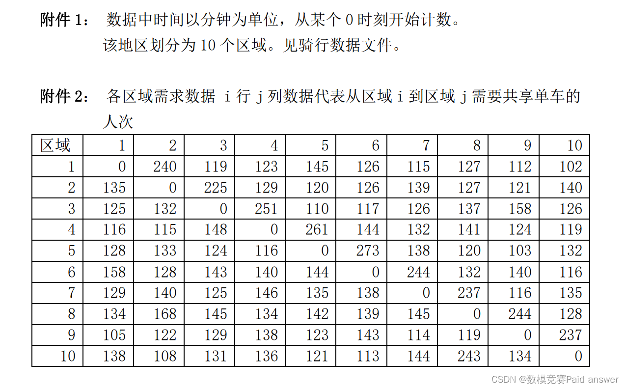
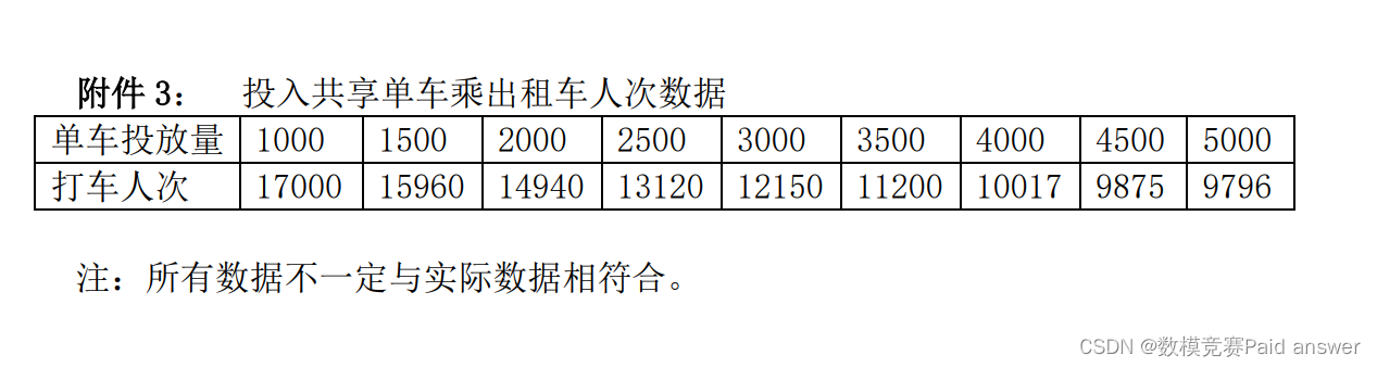
  For question one, we divide the discussion into time distribution and space distribution. From the perspective of time distribution, bicycles in various regions flow frequently and are densely distributed during 420-900 minutes, and gradually decrease in other periods, and the distribution tends to be static after 1380 minutes. In terms of spatial distribution, we obtained the OD matrix of trains from the departure area to the arrival area through statistical analysis of VBA programming. The distribution between them is relatively dense, and the distribution in other areas is basically uniform.
  Aiming at the second problem, a single dispatching center dispatching model and a dynamic dispatching optimization model are established. According to the data in Annex 1 and Annex 2, calculate the demand for bicycles in each region when there are bicycles, and determine the demand time and acceptable time for bicycles in different regions. Estimate the shortest distance between different regions according to the results of problem 1, establish a single dispatch center dispatch model and use MATLAB software and genetic algorithm to solve the initial dispatch plan, the optimal dispatch route is 2-5-6-3-7-10-9 -2. Based on the soft time window scheduling model of a single dispatch center, a dynamic demand scheduling optimization model is established, new scheduling requirements are continuously inserted into the initial static optimization solution, and the method of "initial static optimization + real-time dynamic optimization" is applied to multiple continuous static scheduling problems Solve and optimize the scheduling route continuously. The initial optimization result is 5-2-3-4-8-10-9, of which 5, 2, and 3 have been dispatched.
  For question three, it is necessary to judge the degree of satisfaction of shared bicycles required in each area. First, we define the demand, satisfaction and demand-satisfaction ratio from departure area i to arrival area j as indicators to measure the degree of satisfaction of shared bicycles in each area. According to the OD matrix obtained in Question 1 and the demand matrix given in Appendix 2, the demand satisfaction ratio from departure area i to arrival area j can be calculated, and then the satisfaction degree of shared bicycles required in each area can be judged. It can be seen from the results that the degree of satisfaction in each region ranges from 78% to 99%. Overall, the degree of satisfaction is relatively good. According to the demand ratio of question 2, the delivery plan of 100 bicycles can be obtained.
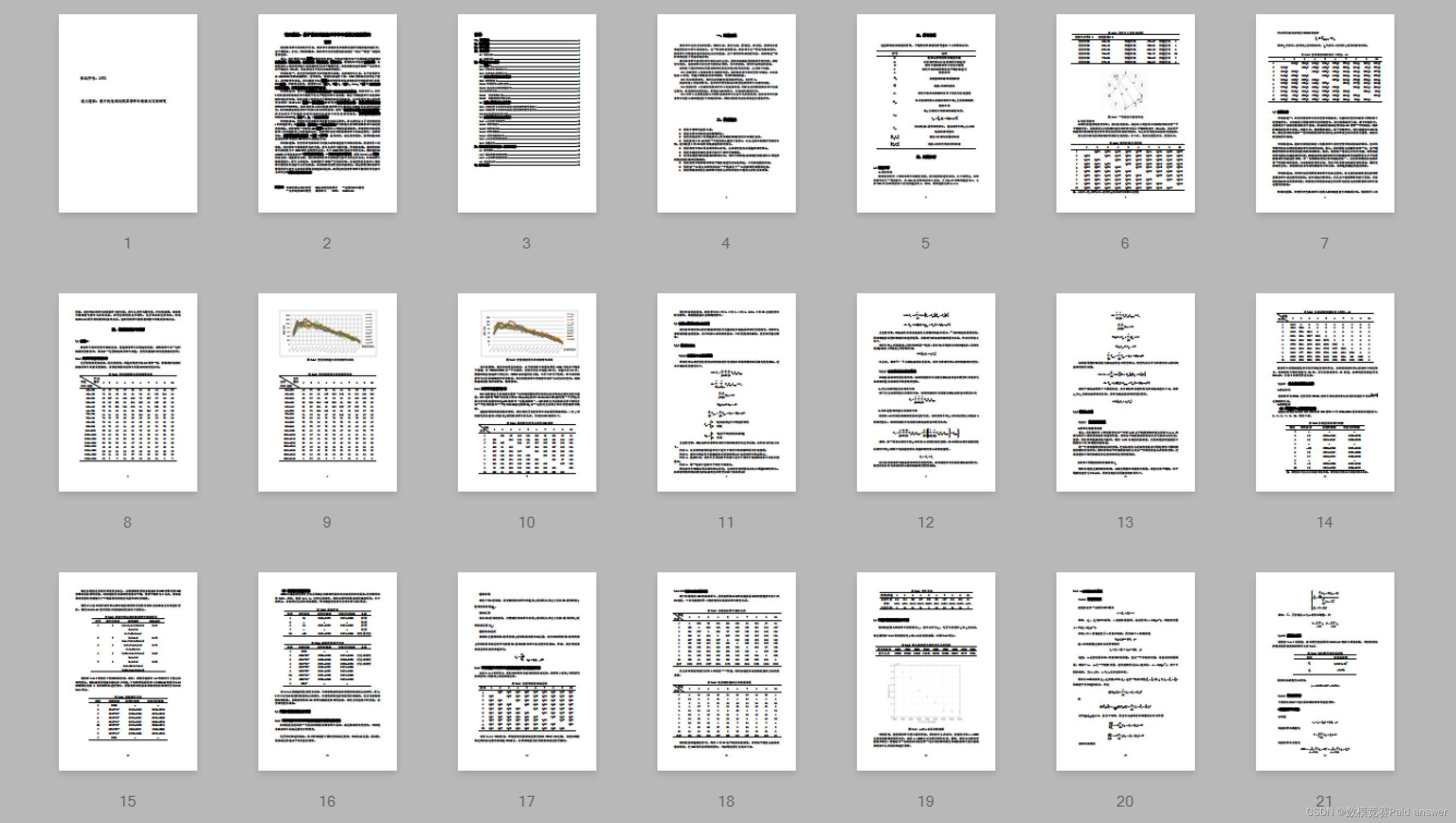
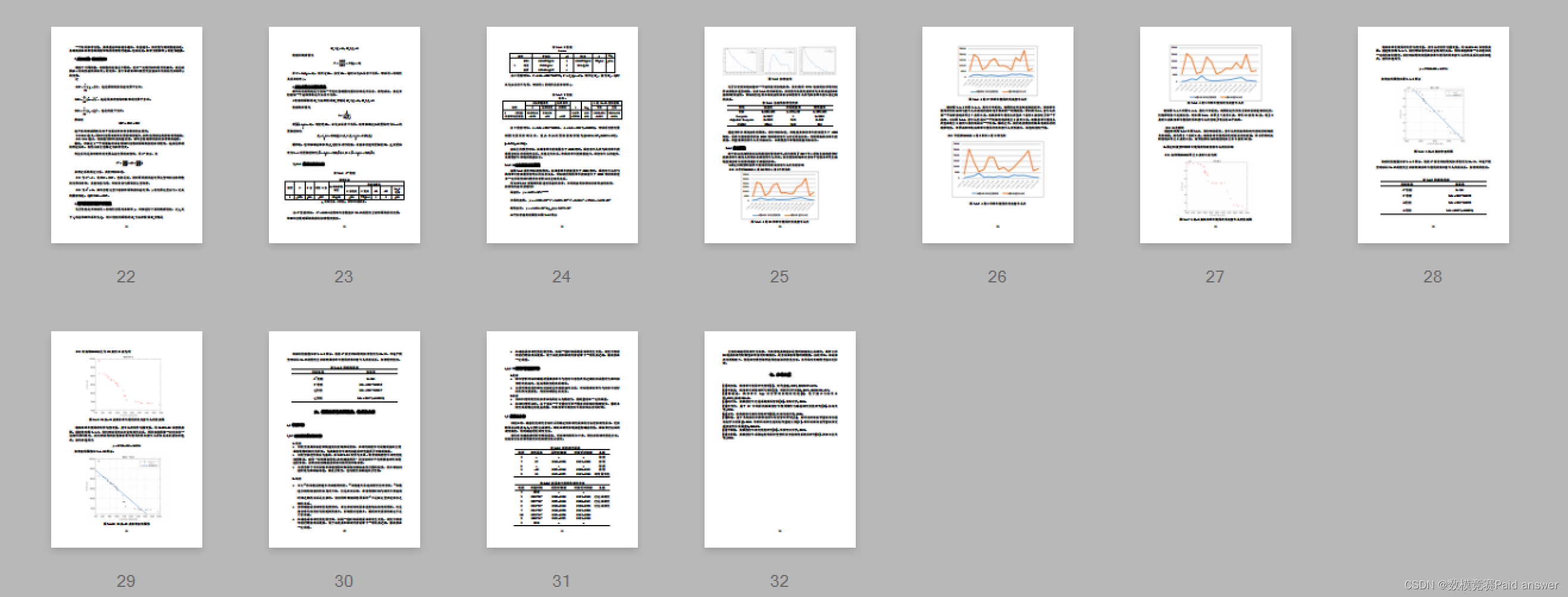
  For question 4, it is necessary to analyze and study the impact of investment in shared bicycles on the taxi-hailing market in the region. According to the data in Appendix 3, we take the number of bicycles as the independent variable and the number of taxis as the dependent variable to make a scatter diagram. It is observed that when the number of bicycles is less than 4000, it shows a linear relationship, and when it is more than 4000, it shows a nonlinear relationship. Therefore, we set up a linear regression model and a nonlinear regression model with x=4000 as the segmentation point, and use MATLAB to solve the equation to obtain the equation. By observing the equation, we can conclude that the amount of shared bicycles is negatively correlated with the number of rides, that is, the greater the amount of shared bicycles, the fewer the number of rides, which will have a negative impact on the ride-hailing market. In addition, we collected data on the number of bicycles used and the number of people who took taxis in April in Shanghai. From the analysis of the time dimension, we can conclude that the images of the number of bicycles used by fixed dates and time intervals and the number of people who took taxis showed similar trends, while the images of the number of bicycles used by fixed periods by date There is a linear negative correlation between the number of rides and the number of rides.

Model assumptions:

  ❖ Assume that 0 minutes is 0:00 in the morning;
  ❖ Assume that the driving speed of each bicycle is uniform and fixed;
  ❖ Assume that the relative distance from departure area i to arrival area j = riding time × riding speed.
  ❖ Assume that there is only one dispatch center in area 1 to 10 and it is located in area 1, equipped with enough dispatch vehicles of the same type to provide dispatch services for all locations in area 1 to 10; ❖ Assume that dispatch vehicles must depart from the dispatch center to complete dispatch
  tasks Then it needs to return to the dispatch center;
  ❖ Assume that the dispatch demand of each region cannot be greater than the dispatching vehicle capacity;
  ❖ Assuming that the shortest network distance between each region is known, dispatching vehicles must choose the shortest road network path between the two regions when driving between any two regions ;
  ❖ Assume that the average driving speed of the dispatched vehicle in the road network is known and fixed, and will not be affected by other factors;
  ❖ Assume that the last location where dispatching was completed in the previous △t is the starting point of the new dispatching route in the next △t;
  ❖ Assume that the collected number of bicycle users and taxi users in Shanghai is true and reliable.

problem analysis:

  For problem 1, when analyzing the spatio-temporal distribution of shared bicycles, it is considered that space-time can refer to both the spatial distribution at different times and the temporal distribution of bicycles in different regions. We consider it comprehensively. For the time distribution, it is not intuitive to directly make a scatter diagram of each point, so we divide it into a time period of every 60 minutes, count the number of bicycle departures and arrivals in the time period, and draw a chart to observe . For the spatial distribution, we establish the OD matrix to describe the travel traffic volume between the origin and destination of all trips within a certain time range in the inter-regional traffic, which indirectly reflects the spatial distribution.
  For question 2, the question requires that a mathematical model be established to solve the problem of how to optimize the scheduling of shared bicycles based on the estimated results of the space-time distribution of shared bicycles in question 1. First, assuming that the cyclist’s cycling distance is constant, the relative distance between each region can be calculated from the average cycling time. Secondly, according to whether the customer demand changes in real time, the scheduling problem can be divided into static and dynamic scheduling problems. When solving the dynamic scheduling problem, the dynamic scheduling problem can be transformed into multiple continuous static scheduling problems for solution, that is, "initial static optimization + real-time dynamic optimization". Firstly, an initial scheduling plan is formed according to the scheduling requirements of each location in the system at a certain moment, and then the scheduling requirements of each location are continuously updated, and the scheduling plan is updated at the same time to realize continuous feedback of scheduling requirements and scheduling paths, and finally achieve the goal of dynamic optimization .
  For question three, it is necessary to judge the degree of satisfaction of shared bicycles required in each area. First of all, we should measure the indicators of the degree of satisfaction of shared bicycles required by each region and establish an index evaluation system. However, due to the incomplete data given in the title, we cannot obtain the specific data of the indicator system, so we only use the demand satisfaction ratio as a measure of the requirements of each region. An indicator of the degree of satisfaction with the need for shared bicycles.
  For question 4, it is necessary to analyze and study the impact of investment in shared bicycles on the taxi-hailing market in the region. According to the data in Appendix 3, we can take the number of bicycles as the independent variable and the number of taxis as the dependent variable, and make a scatter plot to observe the relationship between the number of bicycles and the number of taxis, and explore whether it is linear or nonlinear, positive or negative. Then use MATLAB software to get the specific functional relationship. Then, the relationship between the amount of bicycles put in and the taxi-hailing market is obtained.

Model establishment and solution Overall paper thumbnail

For all papers, please see below "Only modeling QQ business cards" Click on the QQ business card

Program code: (code and documentation not free)

The actual procedure is shown in the screenshot

import pandas as pd
from math import radians, cos, sin, asin, sqrt,ceil
import numpy as np
import geohash

#数据读取
data = pd.read_csv("./mobike_shanghai_sample_updated.csv")
print(data.head(10))
print(data.info())
data['start_time'] = pd.to_datetime(data['start_time'])
data['end_time'] = pd.to_datetime(data['end_time'])
print(data.info())
data["lag"] = (data.end_time - data.start_time).dt.seconds/60
def geodistance(item):
    lng1_r, lat1_r, lng2_r, lat2_r = map(radians, [item["start_location_x"], item["start_location_y"], item["end_location_x"], item["end_location_y，"]]) # 经纬度转换成弧度
    dlon = lng1_r - lng2_r
    dlat = lat1_r - lat2_r
    dis = sin(dlat/2)**2 + cos(lat1_r) * cos(lat2_r) * sin(dlon/2)**2
    distance = 2 * asin(sqrt(dis)) * 6371 * 1000 # 地球平均半径为6371km
    distance = round(distance/1000,3)
    return distance
#data按行应用geodistance()得到distance列的数值
data["distance"] = data.apply(geodistance,axis=1)
#通过摩拜单车的踪迹获取每次交易骑行的路径
def geoaadderLength(item):
    track_list = item["track"].split("#")
    adderLength_item = {
    
    }
    adderLength = 0
    for i in range(len(track_list)-1):
        start_loc = track_list[i].split(",")
        end_loc = track_list[i+1].split(",")
        adderLength_item["start_location_x"],adderLength_item["start_location_y"] = float(start_loc[0]),float(start_loc[1])
        adderLength_item["end_location_x"],adderLength_item["end_location_y"] = float(end_loc[0]),float(end_loc[1])
        adderLength_each = geodistance(adderLength_item)
        adderLength = adderLength_each + adderLength
    return adderLength
data["adderLength"] = data.apply(geoaadderLength,axis=1)
data['weekday'] = data.start_time.apply(lambda x: x.isoweekday())
data['hour'] = data.start_time.apply(lambda x: x.utctimetuple().tm_hour)
data['cost'] = data.lag.apply(lambda x: ceil(x/30))
#因数据集仅包含八月份发起的订单数据，故以9月1日为R值计算基准
data['r_value_single'] = data.start_time.apply(lambda x: 32 - x.timetuple().tm_mday) 
# 按每个用户id所有订单日期距9/1相差天数的最小值作为r值
r_value = data.groupby(['userid']).r_value_single.min()    
f_value = data.groupby(['userid']).size()    # 按每个用户id八月累积订单数量作为f值
m_value = data.groupby(['userid']).cost.sum()    # 按每个用户id八月累积消费金额作为m值
#把r值、f值、m值组合成DataFrame
rfm_df = pd.DataFrame({
    
    'r_value':r_value,'f_value':f_value,"m_value":m_value})
rfm_df["r_score"] = pd.cut(rfm_df["r_value"],5,labels=[5,4,3,2,1]).astype(float)
rfm_df["f_score"] = pd.cut(rfm_df["f_value"],5,labels=[1,2,3,4,5]).astype(float)
rfm_df["m_score"] = pd.cut(rfm_df["m_value"],5,labels=[1,2,3,4,5]).astype(float)
#后面*1是为了把布尔值false和true转成0和1
rfm_df["r是否大于均值"] = (rfm_df["r_score"] > rfm_df["r_score"].mean())*1
rfm_df["f是否大于均值"] = (rfm_df["f_score"] > rfm_df["f_score"].mean())*1
rfm_df["m是否大于均值"] = (rfm_df["m_score"] > rfm_df["m_score"].mean())*1
#把每个用户的rfm三个指标统合起来
rfm_df["class_index"] = (rfm_df["R是否大于均值"]*100) + (rfm_df["f是否大于均值"]*10) + (rfm_df["m是否大于均值"]*1) 

def transform_user_class(x):
    if x == 111:
        label = "重要价值用户"
    elif x == 110:
        label = "消费潜力用户"
    elif x == 101:
        label = "频次深耕用户"
    elif x == 100:
        label = "新用户"
    elif x == 11:
        label = "重要价值流失预警用户"
    elif x == 10:
        label = "一般用户"
    elif x == 1:
        label = "高消费唤回用户"
    elif x == 0:
        label = "流失用户"
    return label
rfm_df["user_class"] = rfm_df["class_index"].apply(transform_user_class)
data = data.merge(rfm_df["user_class"], on = 'userid', how = 'inner')

For all papers, please see below "Only modeling QQ business cards" Click on the QQ business card