[DL] Use pytorch to realize linear regression from zero

1. Introduction to Linear Regression

This content is mainly based on the "Hands-on Deep Learning" course taught by Mr. Li Mu, combined with other materials on the Internet and my own understanding.

Linear regression Mushen B station video course link: https://www.bilibili.com/video/BV1PX4y1g7KC

E-book link: https://zh-v2.d2l.ai/chapter_linear-networks/linear-regression.html

1.1 Linear regression

Regression is usually used to represent the relationship between input and output, and it can be used in the field of machine learning to solve prediction problems, such as predicting housing prices. Linear regression is a type of regression based on a few simple assumptions:

• The relationship between the independent variable x and the dependent variable y is linear;
• Allows adding normal noise, such as noise following a normal distribution, etc.

Let's take a practical example: We want to estimate the price of a house in dollars based on its size (square feet) and age (years). In order to develop a model that can predict housing prices, we need to collect a real dataset. This dataset includes sales prices, square footage, and age of houses. In machine learning terminology, this dataset is called the training data set or training set. Each row of data (such as the data corresponding to a housing transaction) is called a sample, which can also be called a data point or a data instance. We call the target we are trying to predict (say predicting house prices) a label or target . The independent variables (area and age) on which the prediction is based are called features or covariates .

1.2 Gradient Descent

Roughly speaking, at the beginning we will set a random weight w0, which corresponds to a set of solutions of the function. Because we need to obtain the optimal solution of the function, we need to let the gradient go in the direction of the optimal solution, and the gradient itself is the direction that makes the function value rise the fastest, so we need to go in the direction of negative gradient, that is, gradient descent :

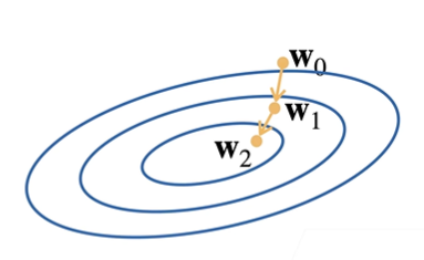
这里我们引入了**学习率 ŋ**（步长的超参数，不能太小也不能太大），它指我们的 w0 沿着负梯度方向每次走多远。如下面公式所示，最右边的项对应着上图中的一个向量，即学习率与**损失函数 l 在上一权重处的梯度**相乘：

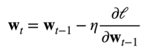
We subtract this vector from the previous weight to get the new weight. The above iterations are repeated, and each iteration is along the direction of the fastest decline of the loss function, and the value of the loss function is getting smaller and smaller, thus approaching the true value.

1.3 Mini-batch stochastic gradient descent

In practice, since calculating the gradient on the entire training set is too resource-intensive and time-consuming, we usually use the mini-batch stochastic gradient descent method. We randomly sample b samples, find the loss value of this batch and average it, so as to approximate the loss.

2. Actual combat

This code comes from Li Mu's "Hands-on Deep Learning" course

The video course link of station b in this section: https://www.bilibili.com/video/BV1PX4y1g7KC

E-book link: https://zh-v2.d2l.ai/chapter_linear-networks/linear-regression.html

My operating environment: ubuntu22.04 + Conda + Python310 + jupyter + pytorch

rely:

%matplotlib inline
import random
import torch
from d2l import torch as d2l

2.1 Dataset Creation

To sum up, before making predictions, we need to create a data set, the code is as follows:

def synthetic_data(w, b, num_examples):
    X = torch.normal(0, 1, (num_examples, len(w)))
    y = torch.matmul(X, w) + b
    y += torch.normal(0, 0.01, y.shape)
    return X, y.reshape((-1, 1))

# 人为设置 w 和 b 的真实值
true_w = torch.tensor([2, -3.4])
true_b = 4.2
features, labels = synthetic_data(true_w, true_b, 1000)

Among them, w represents the weight of the model (here is a column vector), b represents the bias (here is a scalar), in the real case, w and b are unknown. Since high-dimensional datasets are commonly used in machine learning , they are usually constructed using vectors or tensors. The predicted value y is expressed as follows:

$y=Xw+b+e$

• X generated as a random tensor with mean=0, standard deviation=1, num_examples rows, len(w) columns

• y is calculated according to the above linear regression formula and returned as a column vector.

  Here b is a one-dimensional vector. When the first parameter of matmul is a two-dimensional vector and the second parameter is a one-dimensional vector, the product of the matrix and the vector is returned, and the result is a vector (from the barrage of station b). Therefore, y needs to be reshaped as a column vector, where -1 means automatic calculation.

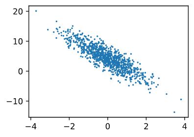
• We set the linear model parameters to w = [2, -3.4] ^T , b = 4.2, and save the results as features and labels

  Note that featureseach row in contains a two-dimensional data sample, and labelseach row in contains one-dimensional label values ​​(a scalar).

By generating a scatter plot of featuresand labels, you can visually observe the linear relationship between the two:

d2l.set_figsize()
d2l.plt.scatter(features[:, (1)].detach().numpy(), labels.detach().numpy(), 1);

2.2 Read the dataset

Usually in machine learning, when training a model, we need to traverse the data set, take a small batch of samples each time, and use them to update our model.

In order to mimic the above purpose, in the code below, we define a data_iterfunction to shuffle the samples in the dataset and get the data in small batches. The function receives as input a batch size, a feature matrix, and a label vector, and generates a batch_sizemini-batch of size . Each mini-batch contains a set of features and labels.

def data_iter(batch_size, features, labels):
    num_examples = len(features)
    # 生成索引列表
    indices = list(range(num_examples))
    # 打乱索引列表
    random.shuffle(indices)
    for i in range(0, num_examples, batch_size):
        batch_indices = torch.tensor(
            indices[i: min(i + batch_size, num_examples)])
        yield features[batch_indices], labels[batch_indices]

Note: The function with the yield keyword is a generator, which is similar to return. When the program executes to yield, return returns the generated number, and when it enters iteration, it starts from the place where the previous step stopped, that is, after yield.

We set the mini-batch to 10 (not too small or too large), and then start to iteratively generate X, y after mini-batch processing. Due to the large amount of data, here we only print it once:

batch_size = 10

for X, y in data_iter(batch_size, features, labels):
    print(X, '\n', y)
    break

The result is:

tensor([[ 0.3145,  0.1654],
        [ 2.0859, -1.2568],
        [ 0.3655,  1.1703],
        [ 0.8599, -0.6612],
        [ 0.3118, -0.4277],
        [ 1.3142,  0.3179],
        [ 0.2688, -0.6435],
        [-1.5495,  0.4066],
        [-0.3208, -0.5531],
        [-1.7611,  0.4214]]) 
 tensor([[ 4.2507],
        [12.6318],
        [ 0.9561],
        [ 8.1628],
        [ 6.2739],
        [ 5.7383],
        [ 6.9305],
        [-0.2778],
        [ 5.4270],
        [-0.7713]])

This is our first batch of data.

2.3 Initialize the model

First initialize the parameters of the model:

w = torch.normal(0, 0.01, size=(2, 1), requires_grad=True)
b = torch.zeros(1, requires_grad=True)
lr = 0.03
num_epochs = 3

We initialize the weight as a random two-dimensional column vector with mean=0, standard deviation=0.01, 2 rows and 1 column, because we need to calculate the gradient, so requires_grad=True.

The bias is directly set to scalar 0, the learning rate is 0.03, and the iteration period is set to 3, that is, three rounds of training are performed.

Afterwards, create the linear regression model:

def linreg(X, w, b):
    """线性回归模型"""
    return torch.matmul(X, w) + b

2.4 Define the loss function

def squared_loss(y_hat, y):
    """均方损失"""
    return (y_hat - y.reshape(y_hat.shape))**2 / 2

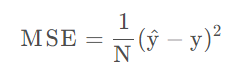
About the mean square loss (Mean Squared Error, MSE) :

The mean square error loss function is the mean value of the sum of squares of the corresponding point errors of the predicted data and the original data, and the formula is:

N is the number of samples.

Quoted from: https://blog.csdn.net/qq_40210586/article/details/115470696

In our implementation, we need to ytransform the shape of the ground truth to be y_hatthe same shape as the predicted value

2.5 Mini-batch stochastic gradient descent

Define an optimization algorithm that implements mini-batch stochastic gradient descent updates. The function accepts as input a set of model parameters, a learning rate, and a batch size. The size of the update at each step lris determined by the learning rate. Because the loss we compute is the sum of a batch of samples, we batch_sizenormalize the stride size by the batch size ( ) so that the stride size does not depend on our choice of batch size.

def sgd(params, lr, batch_size):
    """小批量随机梯度下降"""
    with torch.no_grad(): # 不计算梯度
        for param in params: # 更新参数
            param -= lr * param.grad / batch_size
            param.grad.zero_() # 将梯度设置为0，防止与下一个梯度相关

Note:

Since the parameter passed in the sgd function is a multi-dimensional list composed of w and b, param gets a reference to the elements in the list when passing, so changing param inside the function will also change w and b outside.

At the same time, it should be noted that when the parameter is updated, the -= operator is used to perform an in-place operation (in-place operation), that is, the operation result will be assigned to the same block of memory. If it is modified to the form of param = param - ..., the test code is as follows:

        for param in params:
            print(type(param), 'id:', id(param))
            param -= lr * param.grad / batch_size
            print(type(param), 'id:', id(param))
            param = param - lr * param.grad / batch_size
            print(type(param), 'id:', id(param))

The result is as follows:

<class 'torch.Tensor'> id: 140296289112448
<class 'torch.Tensor'> id: 140296289112448
<class 'torch.Tensor'> id: 140295014093344

It can be seen that param is stored in a new memory space, so the value of the global variable cannot be changed.

In each iteration cycle, we use data_iterthe function to traverse the entire data set, take out the small batch data X, y from it, put X into the linear regression model to calculate the predicted value, and then put the predicted value and the real value into the loss function, Find the mini-batch loss.

net = linreg
loss = squared_loss

for epoch in range(num_epochs):
    # 更新参数
    for X, y in data_iter(batch_size, features, labels):
        l = loss(net(X, w, b), y) # 计算 X 和 y 的小批量损失
        l.sum().backward()
        sgd([w, b], lr, batch_size) # 更新梯度
    # 测试使用更新后的w和b得到的损失
    with torch.no_grad():
        train_l = loss(net(features, w, b), labels)
        print(f'epoch {
      
      epoch + 1}, loss {
      
      float(train_l.mean()):f}')

The result is:

epoch 1, loss 0.037120
epoch 2, loss 0.000136
epoch 3, loss 0.000048

About backward()the method:

That is, the backpropagation function, which is used for reverse derivation. For example, after executing the above code l.sum().backward(), execute again w.gradto obtain the derivative of the loss function with respect to w, that is, the gradient.