Many books about TF development like to use logistic regression to fit linear two-dimensional data to start the development process of TF. According to data preparation, model building, reverse loss function definition and training model, the order of using the model is introduced. And give the code. But the TF framework itself hides most of the processes and only exposes a small part of the parameters for the user program to adjust, causing the learner to know it but not knowing why. It may be that a short line of tf function call hides most of the Implementation details. According to the information of online learning, combined with my own exploration, here is an example of implementing a linear function fitting with a single neuron without relying on tensorflow, which is also implemented in python. On the one hand, I do this because I am also a novice, and the process of writing is a learning process, which can deepen the impression. On the other hand, if there is something wrong in it, it can be pointed and corrected by others.
Single neuron working model:
For conformity like
![]()
The data of this kind of linear function distribution can theoretically be fitted by a single neuron. The working model of a single neuron is as follows:
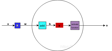
The functions completed by the network are briefly introduced as follows, x is the sample input, w is the weight, the middle square box indicates that the operation between x and w is a multiplication operation, and then the result is added to the subsequent b, and the result y is in a process called The transformation of the activate function function, the final output is obtained o. l The above calculation process is expressed by the equation as follows:
In the field of neural networks, professionally called b as bias, w as weight, and f as activation function, also called nonlinear unit
The process of fitting is simply to continuously adjust the weight w and bias b according to the error trend of the output value and the expected value through continuous input samples to obtain the best weight and replacement value suitable for the sample data. This process is the training process .
In addition, I would like to add a digression. I learned automation. The word that I have most contact with in automation majors is "negative feedback". The neural network working process described above actually uses the principle of feedback to divide the expected value and the actual value. The error is used as the control signal source, through the network "feedback" to the previous neuron node, to generate the control signal to control the change of w and b, so as to make the output and the expected value fitting process. The commonly used BP neural network, BP (back propagate, negative propagation) is also in harmony with the principle of negative feedback, and the control variable corresponding to the negative feedback becomes a negative gradient.
Based on the above network model, the implementation of data fitting with noise in accordance with the y=6x law is given below.
data preparation:
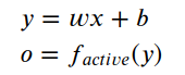
The following code generates a set of 100 samples in the interval [-1,1], and multiplies each sample value by 6 and adds random noise to output.
import numpy as np
import matplotlib.pyplot as plt


traing_x=np.linspace(-1, 1, 100)
traing_y=6*traing_x + np.random.randn(*traing_x.shape) * 0.3

plt.plot(traing_x,traing_y,'ro', label='Original data')
plt.legend()
plt.show()
The data image is:
According to the data image distribution, it is generally consistent with
![]()
The distribution law of noise causes the data points to fluctuate within a range not far from the straight line.
Select activation function:
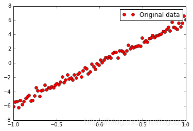
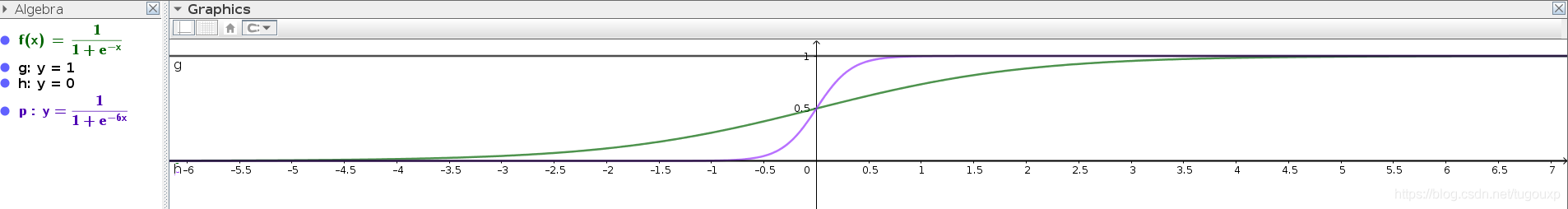
Choose the more commonly used sigmoid function as the activation function, and its image is:
Another reason for choosing it as the activation function is that it can be seen from the data distribution graph that the value range of x is [-1,1], the value range of y is [-6,6], and the sigmoid function is in [ -6,6] The interval has a relatively good degree of discrimination.
After checking the function, the transfer equation of the above neural network:
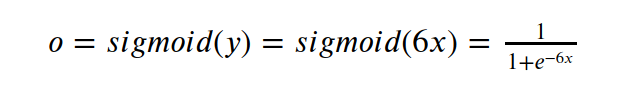
The image becomes as follows:
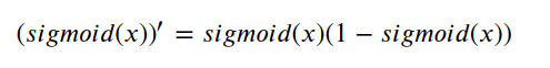
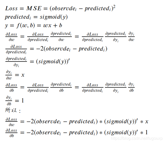
The network train is carried out according to the negative gradient. The calculation process of the negative gradient is the partial derivative of the loss function with respect to the weight and bias. According to the chain derivation rule, the sigmoid function derivation is the middle part of the chain rule. The following is the calculation sigmoid derivative process

Therefore, the derivative of the sigmoid function is:
Choose loss function:
Here we choose Mean Squared Error (MSE), also known as "Mean Squared Error" as the evaluation index of the training result, that is, the loss function, which mainly expresses the difference between the predicted value and the true value. In mathematical statistics Among them, the mean square error refers to the expected value of the square of the difference between the estimated value of the parameter and the true value of the parameter. It is defined as follows:
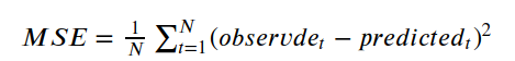
The predicted value and the true value are the output after mapping by the sigmoid function.
Take single training as an example. In this example, each single data of each training period is a sample:

The purpose of training optimization is to continuously reduce the value of the loss function. We know that changing the weight and bias of the network can affect the predicted value, but what should we do to optimize the result in the direction of the loss function reduction? Some concepts in advanced mathematics are needed here.
Observde is the true value of the sample, which is a constant that belongs to the external input of the model, and there is no need to derive it. Therefore, the partial derivatives of w and b are respectively calculated as
Model building:
Define activation function, loss function, sigmoid derivation function and other subroutines:
# Sigmoid activation function: f(x) = 1 / (1 + e^(-x))
def sigmoid(x):
    return 1 / (1 + np.exp(-x))

# Derivative of sigmoid: f'(x) = f(x) * (1 - f(x))
def derivative_sigmoid(x):
    f = sigmoid(x)
    return f * (1 - f)

def mse_loss(expect, actual):
    return ((expect - actual) ** 2).mean()
Then define the neuron, where the derivative is calculated according to the formula given above, but what about updating the new w, b values according to the partial derivative? The concept of negative gradient is used here.
According to the above formula, the gradient of the loss function is:
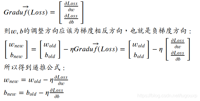
As for why the negative gradient is chosen, you can think of it like this:
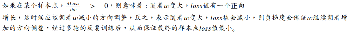
Among them is the declining rate of change of the gradient descent algorithm, which is used to control the convergence speed of the gradient algorithm. There is a special name in machine learning, called the learning rate, which can be a number between 0 and 1. When the local optimum is obtained After the bias and weight of, the gradient vector becomes 0, and the recursive formula obtains a stable output. At this time
The algorithm reaches the optimal solution.
class one_neural_network:
  def __init__(self):
    # Weights
    self.w = np.random.normal()
    # Biases
    self.b = np.random.normal()


  def feedforward(self, x):
    # x is a numpy array with 2 elements.
    o= sigmoid(self.w * x + self.b)
    return o

  def train(self, input, expect):
    learn_rate = 0.1
    epochs = 600 # number of times to loop through the entire dataset
    datasets = traing_x.shape[0];

    result = np.zeros(epochs)
    for epoch in range(epochs):
      for counter in range(datasets):
        x=traing_x[counter]
        y=traing_y[counter]

        o1 = self.w * x + self.b
        o2 = sigmoid(o1)

        exp = sigmoid(y)
        d_L_d_input = -2 * (exp - o2)
        d_input_d_w = x * derivative_sigmoid(o1)
        d_input_d_b = derivative_sigmoid(o1)

        self.w -= learn_rate * d_L_d_input * d_input_d_w
        self.b -= learn_rate * d_L_d_input * d_input_d_b

      y_predict = np.apply_along_axis(self.feedforward, 0, traing_x)
      loss = mse_loss(sigmoid(traing_y), y_predict)
      print("Epoch %d loss: %.3f" % (epoch, loss))
      result[epoch] = loss;
    print(self.w)
    print(self.b)
    plt.plot(result)
    plt.grid(True)
    plt.axis('tight')
    #plt.ylim(0,0.1)
    plt.show()
Write application code:
The application code is actually very simple, they are all direct calls to the functions that have been encapsulated above, just feed the model data to these functions.
# train our neural network!
network = one_neural_network()
network.train(traing_x, traing_y)
Perform training:
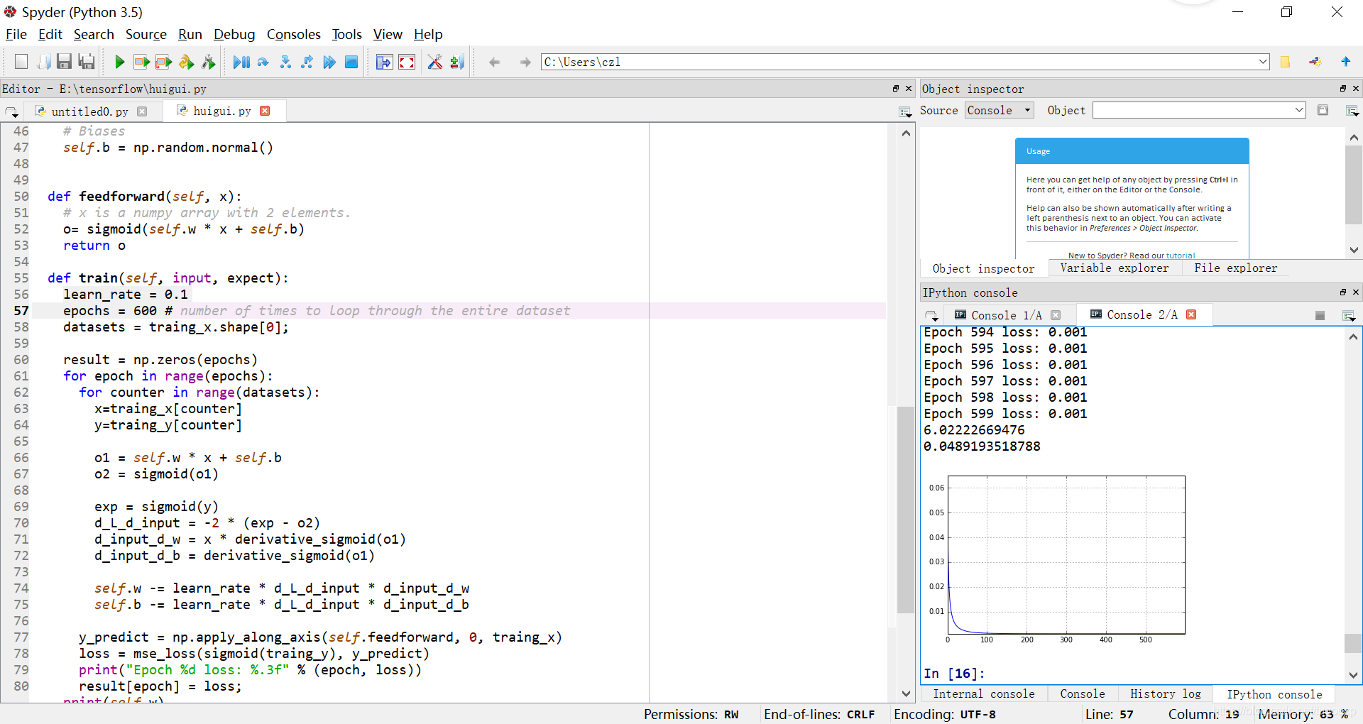
The learning rate is set to 0.1 in the program, 600 rounds of training, after 600 rounds of training, the results obtained are as follows:
Epoch 595 loss: 0.001
Epoch 596 loss: 0.001
Epoch 597 loss: 0.001
Epoch 598 loss: 0.001
Epoch 599 loss: 0.001
6.02222669476
0.0489193518788
Loss curve:
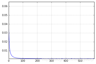
It can be seen from the data that after 600 rounds of training, the average loss is stable and then 0.001. It is also obvious from the loss curve that as the training progresses, the MSE loss becomes smaller and smaller.
In the end, the trained w=6.02222669476 and b=0.0489193518788 are very close to the true values of 6 and 0.
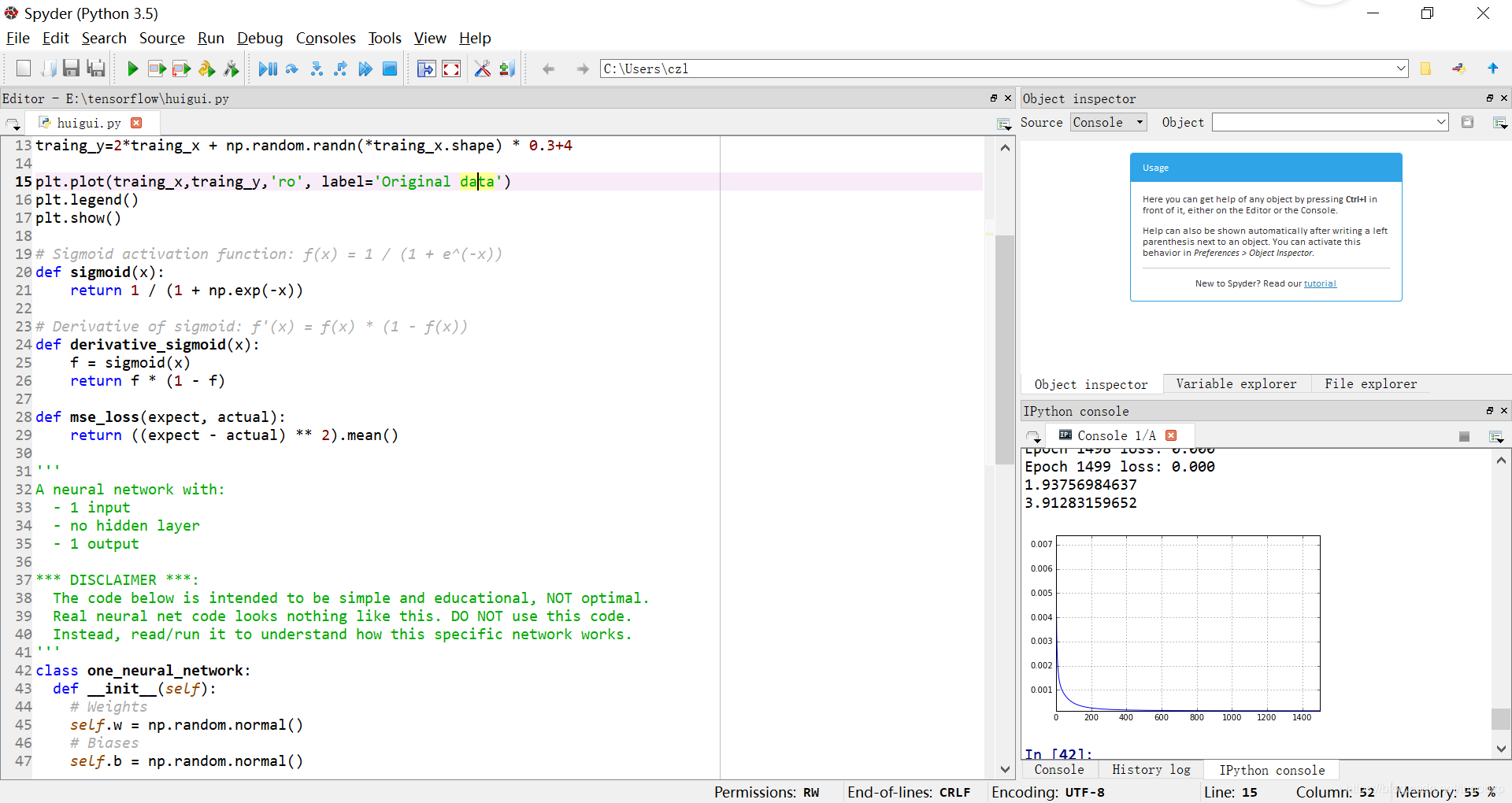
Further, modify the model function, adjust the w and b values of the initial data to see if the above code can track the new changes, let b=4, w=2, and adjust the training for 1500 rounds.
traing_y=2*traing_x + np.random.randn(*traing_x.shape) * 0.3+4Change graph of loss function:
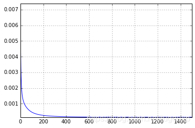
Epoch 1496 loss: 0.000
Epoch 1497 loss: 0.000
Epoch 1498 loss: 0.000
Epoch 1499 loss: 0.000
1.93756984637
3.91283159652
It is worth noting that the value of the learning rate has a great influence on the training effect. An inappropriate learning rate may even cause the loss function to not converge. With a suitable learning rate, the loss function will be reduced in each iteration, as shown in the image The middle is that the loss function presents a monotonously decreasing form as the number of iterations increases.
Mathematicians have proved that as long as the learning rate is set small enough, the loss function will definitely converge, but the speed of convergence is fast or slow, so if you encounter a situation of non-convergence, the most likely reason is that the learning rate is set too large.
It can be seen that w converges to 1.93796984637, b converges to 3.91231596552, which is very close to 2 and 4, and the loss value is close to 0, and the error is basically undetectable.
The above is the principle of regression training in the TF framework. Although not necessarily the same, the thinking should be the same.
Attached
After performing the learning, it is time to infer, enter a new value of x, and it will give you the most realistic output.