Simple Linear Regression Using Pytorch

Our task is to give some data points, which are composed of a linear function plus noise. We need to get the parameters of the function once through training.
The formula for the data is
$$y=wx+b+c$$
where y is the final data, w and b are the parameters we need, and c is the noise.

Step 1: Generate a dataset

We randomize a list of x, use a real w and b to calculate its corresponding y value, add a noise to the y value, and use the noised data as our training data.

%matplotlib inline   
#此语句可以让plot绘制的图直接显示在jupyter 的控制台里
import torch
from IPython import display
from matplotlib import pyplot as plt
import numpy as np
import random

num_inputs = 2
num_examples = 1000
true_w = [2,-3.4]
true_b = 3.2
features = torch.from_numpy(np.random.normal(0,1,(num_examples,num_inputs)))
labels = true_w[0] * features[:,0] + true_w[1] * features[:,1] + true_b  #生成正确的数据,这里是y

#给正确的数据加一点噪声
labels += torch.from_numpy(np.random.normal(0,0.01,size = labels.size()))  #np.random.normal参数：均值  标准差  输出的矩阵大小

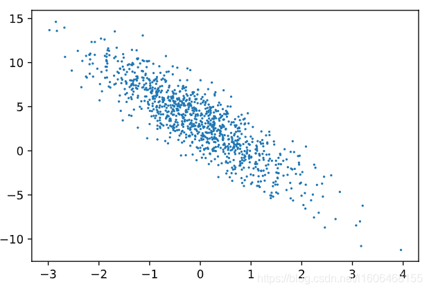
plt.scatter(features[:,1].numpy(),labels.numpy(),1);

Here we generate 1000 values ​​and draw its graph as follows:

Define data reading function

Next, let's define a data reading function, which is to randomly read a batch of data from the data set we generated each time

#数据读取函数，每次从features和labels中随机读取一个批次的数据
def data_iter(batch_size,features,labels):
    num_examples = len(features)
    indices = list(range(num_examples))
    random.shuffle(indices)  #随机排列样本
    for i in range(0,num_examples,batch_size):
        j = torch.LongTensor(indices[i:min(i + batch_size,num_examples)])   #将下标切片，并转换成LongTensor类型赋给j
        
        yield features.index_select(0,j),labels.index_select(0,j)

Initialize model parameters

The type of setting in the original book here is torch.float32, but the data generated earlier is all torch.float64, and the matrix multiplication later will report an error due to inconsistent types. Here, it is changed to torch.float64

w = torch.tensor(np.random.normal(0,0.01,(num_inputs,1)),dtype = torch.float64)
b = torch.zeros(1,dtype = torch.float64)
# w.requires_grad = True
# b.requires_grad = False
#上面直接设置或者使用原地处理方式
w.requires_grad_(requires_grad = True)
b.requires_grad_(requires_grad = True)

define model

Here is actually a calculation function defined to calculate $y_1$It is convenient to calculate the error from the real value later.

def linreg(x,w,b):#这里使用的torch.mm  需要保证x w 和 b类型一致   比如均为torch.float32 或者 均为 torch.float64，如果不一致会报错
    return torch.mm(x,w) + b  # 这里返回的是x与w相乘再加b  实际上即计算y

Define the loss function and optimization method

def squared_loss(y_hat,y):
    return (y_hat - y.view(y_hat.size())) ** 2 / 2    #   a**b 即a的b次方，除2应该是为了后面求导消参数 

#随机梯度下降法
def sgd(params,lr,batch_size):
    for param in params:
        param.data -= lr * param.grad / batch_size   #让其沿着梯度减少

Start training the model

In fact, use w and b to substitute in to calculate $y_1$, and then calculate the loss ( $y_{1}distancefromy)$ , use the optimization function to reduce this loss

lr = 0.03   #学习率
num_epochs = 3 #训练次数
net = linreg #设置网络的操作，也就是前面说的那个计算y值的函数
loss = squared_loss #设置计算损失的方法
for epoch in range(num_epochs):
    for x,y in data_iter(batch_size,features,labels):
        l = loss(net(x,w,b),y).sum()  
        l.backward()
        sgd([w,b],lr,batch_size)#使用优化算法迭代模型参数
        
        #清空梯度
        w.grad.data.zero_()
        b.grad.data.zero_()
    train_l = loss(net(features,w,b),labels)
    print('Epoch %d,loss %f ' %(epoch+1,train_l.mean().item()))

Here is my output here:

Epoch 1,loss 0.030724 
Epoch 2,loss 0.000125 
Epoch 3,loss 0.000049 

Let's compare the real and trained values:

print(true_w,'\n',w)
print(true_b,'\n',b)

The result is:

[2, -3.4] 
 tensor([[ 1.9998],
        [-3.3995]], dtype=torch.float64, requires_grad=True)
3.2 
 tensor([3.1997], dtype=torch.float64, requires_grad=True)

Our real w is set to 2 and -3.4, and the training is 1.9998 and -3.3995. The
real b is set to 3.2, and the training b is 3.1997.
It can be seen that we only trained three times, and the obtained The value is basically in line with the trend, but this is just a very simple model with only two parameters. When our model is very complicated, we need to add more layers for training.

PS.

The above code comes from Github "Hands-on Deep Learning" Pytorch version