Table of contents
1 Pytorch implements linear regression
2 Detailed explanation of each part of the code line by line
2.2.2 Detailed explanation of the code line by line
2.3 Construct loss function and optimizer
3 Commonly used optimizers in linear regression
1 Pytorch implements linear regression
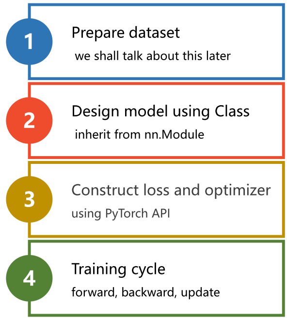
1.1 Implementation ideas
1.2 Complete code
import torch
x_data = torch.Tensor([[1.0], [2.0], [3.0]])
y_data = torch.Tensor([[2.0], [4.0], [6.0]])
class LinearModel(torch.nn.Module):
    def __init__(self):
        super(LinearModel, self).__init__()
        self.linear = torch.nn.Linear(1, 1)
    def forward(self, x):
        y_pred = self.linear(x)
        return y_pred
model = LinearModel()
criterion = torch.nn.MSELoss(size_average=False)
optimizer = torch.optim.SGD(model.parameters(), lr=0.01)
for epoch in range(500):
    y_pred = model(x_data)
    loss = criterion(y_pred, y_data)
    print(epoch, loss.item())
    optimizer.zero_grad()
    loss.backward()
    optimizer.step()
print('w = ', model.linear.weight.item())
print('b = ', model.linear.bias.item())
x_test = torch.Tensor([[4.0]])
y_test = model(x_test)
print('y_pred = ', y_test.data)
2 Detailed explanation of each part of the code line by line
2.1 Prepare the dataset
In PyTorch, it is generally necessary to construct a data set in the form of mini-batch , that is, to define the data set in the form of tensor (Tensor) to facilitate subsequent calculations.
In the following code, x_data is a two-dimensional tensor, which has 3 samples, and each sample has 1 feature value, that is, the dimension is (3, 1) ; y_data is the same. Students who are not clear can use the x.dim() method and the x.shape attribute to obtain the dimension and size of the tensor and debug it by themselves. In short, in a minibatch, rows represent samples and columns represent features
import torch
x_data = torch.Tensor([[1.0], [2.0], [3.0]])
y_data = torch.Tensor([[2.0], [4.0], [6.0]])
2.2 Design Model

Main Goal: Build Computational Graphs
2.2.1 Code
class LinearModel(torch.nn.Module):
    def __init__(self):
        super(LinearModel, self).__init__()
        self.linear = torch.nn.Linear(1, 1)
    def forward(self, x):
        y_pred = self.linear(x)
        return y_pred
model = LinearModel()
2.2.2 Detailed explanation of the code line by line
class LinearModel(torch.nn.Module):Generally, we need a class that inherits from PyTorch's Module class, because it torch.nn.Moduleprovides many useful functions, making it easier for us to define, train and use neural network models.
Next, at least two functions need to be implemented, namely init and forward .
__init__ method
    def __init__(self):
        super(LinearModel, self).__init__()
        self.linear = torch.nn.Linear(1, 1)
This method initializes the parameters of the model .
In super(LinearModel, self).__init__(), the first parameter LinearModel specifies the starting point of the search, which is to search in the parent class of the class; the second parameter specifies the current object, that is, the object calling the method. The function of this statement is to call the method of the parent class and initialize the properties of the parent class. This is a required statement to initialize the model. LinearModelself LinearModel torch.nn.Module__init__
Next an torch.nn.Linearobject is instantiated and assigned to self.linearthe property. torch.nn.LinearThe constructor of receives three parameters: in_features , out_features、bias , which respectively represent the number of input features, the number of output features and the offset.

forward method
    def forward(self, x):
        y_pred = self.linear(x)
        return y_pred
The function of forward() method is to perform feedforward operation, which is equivalent to calculation.
Note that this is equivalent to rewriting the forwardtorch.nn.Linear method in the class . After we override forward , the function will execute as follows:

y_pred = self.linear(x)The function of is to xpass the fully connected layer for linear transformation to obtain the output . y_pred
Finally, call the model by instantiating the LinearModel class
model = LinearModel()2.2.3 Troubleshooting
1. You may have questions, where is the backward process in the code?
Answer: The objects constructed by the torch.nn.Module class will automatically complete the backward process. Module The class and its subclasses automatically build a computational graph during forward pass, and automatically perform gradient calculation and parameter update during backward pass .
For example, self.linear=torch.nn.Linear(1, 1), the linear attribute here gets an instance of the Linear class, and Linear inherits from Module , so the backward will be automatically performed here, so we don’t need to manually find the derivative.
2. y_pred = self.linear(x)Why can linear be directly followed by parentheses?
This involves the knowledge points of callable objects (Callable Object) in python syntax . Adding parentheses after self.linear is equivalent to directly adding parentheses to the object, which is equivalent to implementing a callable object .
In self.linear = torch.nn.Linear(1, 1) , it is equivalent to creating a Module object becausenn.Linearthe class inherits from thenn.Moduleclass.
Then we execute the method y_pred = self.linear(x)这段代码,that is equivalent to calling the Moudle class . __call__
So the method nn.Moduleof the class __call__will further automatically call forwardthe method of the module.
for example:
class Adder:
    def __init__(self, n):
        self.n = n

    def __call__(self, x):
        return self.n + x

add5 = Adder(5)
print(add5(3))  # 输出 8
In this example, we define a Adderclass that takes one parameter nand implements the method. When we create an object , we actually create an object and set to . When we call the object , we actually call the method of the object , __call__ add5Adder n5add5Adder __call__
By implementing __call__the method , we can make the object be called like a function, which is useful in some scenarios, for example, we can use it to implement a state machine, a closure, or a decorator, etc.
3. Where is the weight reflected? Forward does not seem to involve the introduction of weight values?
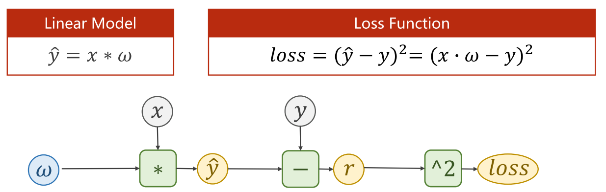
This is self.linearactually a PyTorch module (Module) , which contains the weight matrix and bias vector, so we can use this object to complete the calculation shown in the figure below


So how is the weight passed into forward?
In torch.nn.Linearthe constructor of the class __init__, it automatically creates an nn.Parameterobject for storing the weights and registers them as the learnable parameters of the model (Learnable Parameter) .
The creation code for this nn.Parameterobject is at this line in nn.Linearthe class's function:__init__
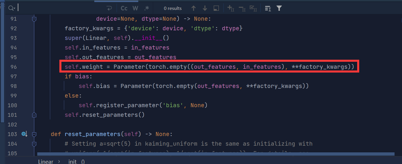
Therefore, the properties self.linearin weightare actually nn.Parameterfetched from the object. In forwardthe method, self.linearits attributes are automatically obtained weightand used to perform matrix multiplication operations.
2.3 Construct loss function and optimizer
criterion = torch.nn.MSELoss(size_average=False)
optimizer = torch.optim.SGD(model.parameters(), lr=0.01)
torch.nn.MSELossis a mean squared error loss function used to calculate the difference between the model output and the true value, or MSE . Among them, size_average the parameter specifies whether to average the loss, and the default is True , that is, to average. In this example, size_average=False it means that we want to get the sum of the squared errors of all samples.

torch.optim.SGDis a stochastic gradient descent optimizer for updating parameters in neural networks. Among them, model.parameters() to optimize the parameters in the neural network, it will check all members and tell the optimizer which parameters need to be updated. During backpropagation, the optimizer computes gradients through these parameters and updates them. lrThe parameter represents the learning rate, which is the step size for each parameter update. In this example, we use stochastic gradient descent as the optimizer with a learning rate of 0.01. Finally we get an optimizer object optimizer .
2.4 Training cycle
for epoch in range(500): # 训练500轮
    y_pred = model(x_data)  # 前向计算
    loss = criterion(y_pred, y_data)  # 计算损失
    print(epoch, loss.item())  # 打印损失值
    optimizer.zero_grad() # 梯度清零,不清零梯度的结果就变成这次的梯度+原来的梯度
    loss.backward()  # 反向传播
    optimizer.step()  # 更新权重
2.5 Test results
The loop iterates for 500 rounds of training.
# Output weight and bias
print('w = ', model.linear.weight.item())
print('b = ', model.linear.bias.item())
# Test Model
x_test = torch.Tensor([[4.0]])
y_test = model(x_test)
print('y_pred = ', y_test.data)
Screenshot of output results:
0 23.694297790527344
1 10.621758460998535
2 4.801174163818359
3 2.208972215652466
4 1.0539695024490356
5 0.5387794971466064
6 0.3084312379360199
7 0.20490160584449768
8 0.1578415036201477
9 0.13593381643295288
10 0.12523764371871948
11 0.1195460706949234
12 0.11609543859958649···
494 0.00010695526725612581
495 0.00010541956726228818
496 0.00010390445095254108
497 0.00010240855044685304
498 0.00010094392928294837
499 9.949218656402081e-05
w = 1.993359923362732
b = 0.015094676986336708
y_pred = tensor([[7.9885]])Process finished with exit code 0
In short, find yhat, find loss, then backward, and finally update the weight
3 Commonly used optimizers in linear regression
• torch.optim.Adagrad
• torch.optim.Adam
• torch.optim.Adamax
• torch.optim.ASGD
• torch.optim.LBFGS
• torch.optim.RMSprop
• torch.optim.Rprop
• torch.optim.SGD
Read more examples from the official tutorial:
Learning PyTorch with Examples — PyTorch Tutorials 1.13.1+cu117 documentation