[Clustering algorithm] spectral clustering spectral clustering

every blog every motto: You can do more than you think.
https://blog.csdn.net/weixin_39190382?type=blog

0. Preface

Spectral clustering spectral clustering overview
description: no

1. Text

1.1 Overall understanding

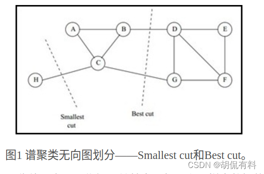
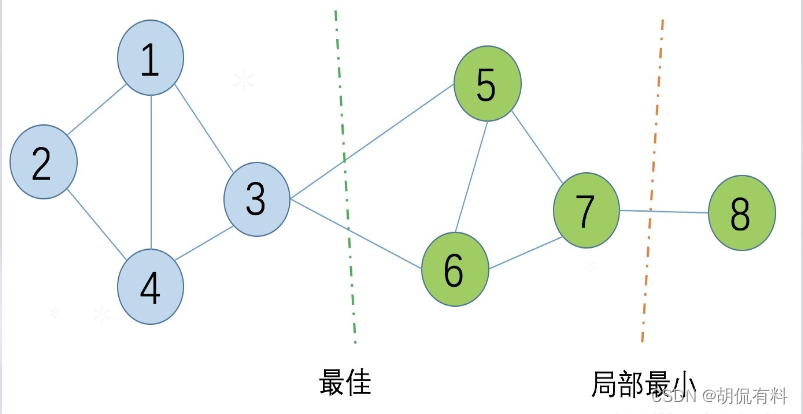
Spectral Clustering is a clustering method based on graph theory, which divides a weighted undirected graph into two or more optimal subgraphs. Make the subgraphs as similar as possible, and the distance between subgraphs as far as possible . The optimal means that the optimal objective functions are different. There are two types:

• smallest cut
• The best cut
  is shown in the figure below:
  

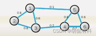
1.1.1 Undirected graph

As shown in the figure below, it consists of several vertices and edges . Because the edges have no direction, it is called an undirected graph. in,

Set of points: $V=\{v1,v2,\_.....,v3\}$
edge set:$E=\{e1,e2,.....,e3\}$

So, the graph is expressed as $G(V,E)$

---

Weight matrix (adjacency matrix) $W$，$W_{ij}$Displayii $i$ and$The\; weight\; between\; j$ , since it is an undirected graph, so
$$W_{ij}=W_{ji}$$

1.1.2 Degree and degree matrix

In data structures, degree is defined as the number of vertices directly connected to the point.
Here, the definition is as follows:
$$d_i=\sum _{j=1}^n{W}_{ij}$$

That is, the sum of weights for a row (or column).
The degree matrix is ​​a diagonal matrix composed of n degrees, as follows:

$$\left[\begin{array}{cccc}{d}_1& 0& \cdots & 0\\ 0& d_2& \cdots & 0\\ ⋮& ⋮& \ddots & ⋮\\ 0& 0& \cdots & d_n\end{array}\right]$$

1.1.3 Similarity Matrix

Note: We can calculate the distance between two points and generate an adjacency matrix to represent the relationship between our points (that is, what we call a graph ). The similarity matrix here is based on the "distance matrix" (according to the distance Judging whether it is similar) According to a certain method (the following three methods) to further "screen"
(it can be roughly understood, some points are far away)

The above weight matrix is ​​composed of weights between any two points. In practice, we cannot directly obtain weights, only the definition of data points, and the weights are usually calculated by the distance between two points . The distance is far away and the weight is high, and the distance is close and the weight is high. Usually by three methods

(1). $ϵ$ - proximity method (less used)

Set a threshold $ϵ$ , calculate the Euclidean distance between two points and compare with the threshold,

$$W_{ij}=\{\begin{array}{ccc}0,& if& s_{ij}>ϵ\\ ϵ& if& s_{ij}⩽\end{array}$$
Use the threshold to filter the distance, the comparison of the card is dead, the weight between the samples is 0, and a lot of information is missing

(2). k-nearest neighbor method

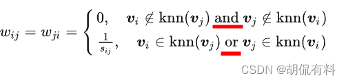
For any point , find the k vertices closest to it, the weights of this vertex and k vertices are obtained by calculation (all are greater than 0, and the distance of the rest of the vertices is 0), but the obtained similarity matrix will be asymmetric. Such as: $i$ in$j$ 'skkAmong the$k$$j$ may not be in$i$ 'skkamong the$k\; nearest\; neighbors.$There are two solutions to this problem:
Description: $s_{ij}$Indicates the distance

a. Method 1

In the loose version,
as long as one satisfies k-nearest neighbors , then let $W_{ij}=W_{ji}$, it is 0 only if k-nearest neighbors are not satisfied at the same time.

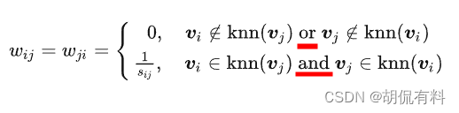
b. Method 2

Strict version Only when
two vertices are close neighbors , the distance is calculated, otherwise the weight is 0.

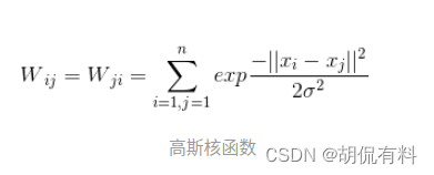
(3). Fully connected

Calculate the interconnection between all points , so the weight is greater than 0, you can choose different kernel functions to calculate the distance, commonly used are:

• polynomial kernel function
• Gaussian kernel function
• sigmoid kernel function

1.1.4 Laplace matrix

$L=D-W$

$D$ is the degree matrix,$W$ is the adjacency matrix above

1.1.5 Cut graph, cluster

Let's get into the key point, now we have to cut the undirected graph mentioned above .

Cut optimization objective:
$$Cost(G1,...G2)=\sum _{i}C(G_i,\widehat{G_i})$$
$$C(G_1,G_2)=\sum _{i\in G_1,j\in G_2}{w}_{ij}$$

• The goal is to minimize the sum of weights for cutting subgraph times , i.e., cut the fewest edges.
• Local optima may appear in cutting, so there are different graph cutting methods according to different cutting methods.

(1). RatioCut

Goal: Make the number of nodes in the subgraph as large as possible
$$RationCut(G1,...G2)=\sum _i\frac{C(G_i,\widehat{G_i})}{\mid \widehat{G_i}|}$$
The denominator is the number of nodes in the subgraph

(2). NCut cut image

Goal: Consider the weight sum of each subgraph edge
$$NCut(C_1,...C_k)=\sum _i\frac{C(G_i,\widehat{G_I})}{vol(\widehat{G_i})}$$

The denominator is the weight sum of each side of the subgraph

1.2 Calculation process

1.2.1 There are three main parts of the core:

• Generation of similarity matrix (commonly used: full connection method)
• Cutting method (commonly used: NCut)
• The final clustering method (commonly used: K-Means)

1.2.2 Algorithm flow:

1. Construct similarity matrix S, degree matrix D, and calculate Laplacian matrix $L=D-W$
2. Construct the standardized Laplacian matrix $D^{\frac{-1}{2}}\cdot L\cdot D^{\frac{-1}{2}}$
3. Calculate $D^{\frac{-1}{2}}\cdot L\cdot D^{\frac{-1}{2}}$The smallest $k_1$The eigenvectors ff corresponding to each eigenvalue$f$
4. The respective eigenvectors $The\; matrix\; composed\; of\; f$ is standardized by row, and the final composition is$n\cdot k_1$The characteristic matrix $F$
5. For each row in F as a $k_1$Dimensional samples, a total of n samples, clustered with the input clustering method, the clustering dimension is $k_2$
6. Get the cluster partition $C(c_1,c_2,...c_{k2})$

1.2.3 python implementation

def calculate_w_ij(a,b,sigma=1):
    w_ab = np.exp(-np.sum((a-b)**2)/(2*sigma**2))
    return w_ab

# 计算邻接矩阵
def Construct_Matrix_W(data,k=5):
    rows = len(data) # 取出数据行数
    W = np.zeros((rows,rows)) # 对矩阵进行初始化：初始化W为rows*rows的方阵
    for i in range(rows): # 遍历行
        for j in range(rows): # 遍历列
            if(i!=j): # 计算不重复点的距离
                W[i][j] = calculate_w_ij(data[i],data[j]) # 调用函数计算距离
        t = np.argsort(W[i,:]) # 对W中进行行排序，并提取对应索引
        for x in range(rows-k): # 对W进行处理
            W[i][t[x]] = 0
    W = (W+W.T)/2 # 主要是想处理可能存在的复数的虚部，都变为实数
    return W

def Calculate_Matrix_L_sym(W): # 计算标准化的拉普拉斯矩阵
    degreeMatrix = np.sum(W, axis=1) # 按照行对W矩阵进行求和
    L = np.diag(degreeMatrix) - W # 计算对应的对角矩阵减去w
    # 拉普拉斯矩阵标准化，就是选择Ncut切图
    sqrtDegreeMatrix = np.diag(1.0 / (degreeMatrix ** (0.5))) # D^(-1/2)
    L_sym = np.dot(np.dot(sqrtDegreeMatrix, L), sqrtDegreeMatrix) # D^(-1/2) L D^(-1/2)
    return L_sym

def normalization(matrix): # 归一化
    sum = np.sqrt(np.sum(matrix**2,axis=1,keepdims=True)) # 求数组的正平方根
    nor_matrix = matrix/sum # 求平均
    return nor_matrix

W = Construct_Matrix_W(your_data) # 计算邻接矩阵
L_sym = Calculate_Matrix_L_sym(W) # 依据W计算标准化拉普拉斯矩阵
lam, H = np.linalg.eig(L_sym) # 特征值分解
    
t = np.argsort(lam) # 将lam中的元素进行排序，返回排序后的下标
H = np.c_[H[:,t[0]],H[:,t[1]]] # 0和1类的两个矩阵按行连接，就是把两矩阵左右相加，要求行数相等。
H = normalization(H) # 归一化处理

model = KMeans(n_clusters=20) # 新建20簇的Kmeans模型
model.fit(H) # 训练
labels = model.labels_ # 得到聚类后的每组数据对应的标签类型
    
res = np.c_[your_data,labels] # 按照行数连接data和labels

1.3 Summary

The main advantages of the spectral clustering algorithm are:

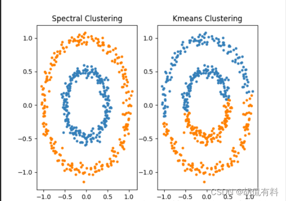
1. Spectral clustering only requires a similarity matrix between the data, so it is effective for clustering dealing with sparse data. This is difficult for traditional clustering algorithms such as K-Means.
2. Due to the use of dimensionality reduction, the complexity of dealing with high-dimensional data clustering is better than traditional clustering algorithms.

The main disadvantages of spectral clustering algorithms are:

1. If the dimension of the final clustering is very high, the running speed of spectral clustering and the final clustering effect are not good due to insufficient dimensionality reduction.
2. The clustering effect depends on the similarity matrix, and the final clustering effect obtained by different similarity matrices may be very different.

reference

[1] https://zhuanlan.zhihu.com/p/387483956
[2] https://blog.csdn.net/songbinxu/article/details/80838865
[3] https://blog.csdn.net/weixin_45591044/article/details/122747024
[4] https://blog.csdn.net/yftadyz/article/details/108933660?ops_request_misc=%257B%2522request%255Fid%2522%253A%2522164345675116780264032305%2522%252C%2522scm%2522%253A%252220140713.130102334…%2522%257D&request_id=164345675116780264032305&biz_id=0&utm_medium=distribute.pc_search_result.none-task-blog-2_alltop_ulrmf~default-2-108933660.pc_search_insert_ulrmf&utm_term=%E8%B0%B1%E5%9B%BE%E7%90%86%E8%AE%BA&spm=1018.2226.3001.4187
[5] https://blog.csdn.net/katrina1rani/article/details/108451882
[6] https://zhuanlan.zhihu.com/p/392736238
[7] https://zhuanlan.zhihu.com/p/91154535
[8] https://www.cnblogs.com/tychyg/p/5277137.html
[9] https://www.cnblogs.com/kang06/p/9468647.html
[10] https://zhuanlan.zhihu.com/p/29849122
[11] https://www.cnblogs.com/xiximayou/p/13548514.html
[12] https://www.cnblogs.com/pinard/p/6221564.html
[13] https://zhuanlan.zhihu.com/p/54348180
[14] https://blog.csdn.net/qq_43391414/article/details/112277987
[15] https://blog.csdn.net/jxlijunhao/article/details/116443245
[16] https://zhuanlan.zhihu.com/p/368878987
[17] https://blog.csdn.net/qq280929090/article/details/103591577