Pooling layer
Responsible for feature selection in CNN , the pooling layer is usually also called subsampling or downsampling. Compress the input feature map (Feature Map), on the one hand, make the feature map smaller, simplify the network calculation complexity and the required video memory; on the one hand, perform feature compression to extract the main features. It is to reduce the input image, reduce pixel information, and only keep important information.
The pooling layer will continuously reduce the space size of the data. It is often used after the convolutional layer to reduce the feature dimension of the output of the convolutional layer through the pooling layer. It can effectively reduce the network parameters and prevent overfitting. .
The function of the pooling layer
Features are not deformed: the pooling operation is that the model pays more attention to whether there are certain features rather than the specific location of the features.
Feature dimensionality reduction: pooling is equivalent to dimensionality reduction in the spatial range, so that the model can extract a wider range of features. At the same time, the input size of the next layer is reduced, thereby reducing the amount of calculation and the number of parameters.
To a certain extent, it prevents overfitting and makes it easier to optimize.
There are four commonly used pooling operations:
1. Average pooling (mean-pooling)
2. Max-pooling
3. Stochastic-pooling
4. Global average pooling
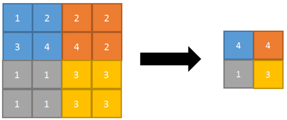
1. Max-pooling
Maximum pooling is a pooling process that uses more, and the advantage is that it can well preserve texture features. Typically, pooling is 2x2 in size.
Maximum pooling process: For the values in a 4×4 feature map neighborhood, use a 2×2 filter to scan with a step size of 2, and select the maximum value to output to the next layer. The maximum pooling process of forward propagation is shown in the figure
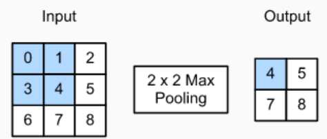
Forward maximum pooling with a step size of 1 is shown in the figure
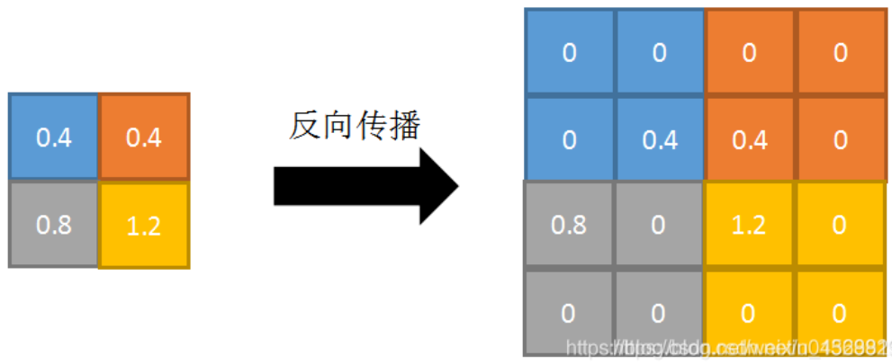
Forward propagation is to take the maximum value in the neighborhood and mark the index position of the maximum value for back propagation.
Backpropagation: Fill the eigenvalues into the forward propagation, the index position with the largest value, and 0 in other positions. As shown below

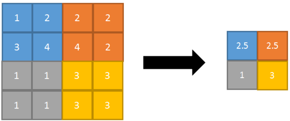
2. Average Pooling
Its characteristic is that it can preserve the background very well, but it is easy to blur the picture. Average pooling process: For the values in a 4×4 feature map neighborhood, use a 2×2 filter to scan with a step size of 2, calculate the average value and output it to the next layer.
The average pooling process of forward propagation is shown in the figure
Backpropagation: The feature values are averaged according to the domain size and passed to each index position. as the picture shows
in the end
Putting the aforementioned convolution, activation, and pooling together forms a simple neural network, and then we increase the depth of the network and add more layers to obtain a deep neural network.

reference: