Deep learning-convolutional neural network CNN

Watch the video:

CNN thought

inspiration

Several problems are often encountered when dealing with image problems:

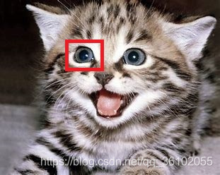
1. We tend to only pay attention to some specific parts when observing images.

For example, for this cat, we don’t need the entire picture to know if the picture has cat eyes, but only a part of it.

For example, you may only need the part in the box below.

2. For a specific area, its location is not fixed.

This is also easy to understand, after all, the cat's eyes in each picture are not necessarily in the same position in the picture.
3. For a picture, we can downsample it.
That is to say, we can do some operations to shrink the picture, thereby reducing the number of input features.

General process

The general working process of CNN is as follows

1. Convolution
2. pooling
3. Repeat 1 and 2 several times
4. Into the fully connected network

convolution

Single channel

Convolution can solve the first and second problems mentioned above.

Each point in a color bitmap is composed of three colors, RGB, and each color can be represented by a two-dimensional matrix.
The three colors need to be represented by a three-dimensional matrix, assuming that the picture is m pixels wide and n pixels wide. Then the information of a color bitmap can be represented by a 3 xnxm three-dimensional matrix.

A bitmap with only black and white colors only needs to be composed of one color, so it must be represented by a 1 xnxm matrix.
We say that this color bitmap has three channels, because there are three nxm matrices used to represent pixel information.
And in black and white, we say he has a channel

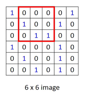
For example, a 6 x 6 black and white picture.

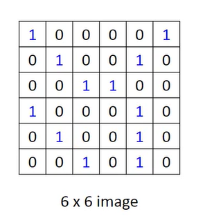
Among them, 1 can mean that there are black blocks, and 0 means that they are white.

The operation of convolution is to first select a fixed size window.

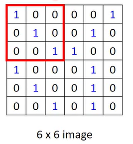
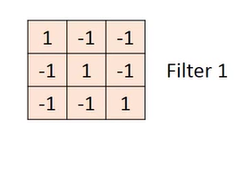
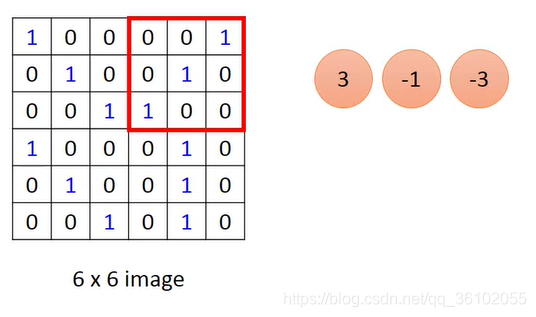
Then the pixel values ​​in this window are correspondingly multiplied by a weight, which is the following matrix, and we will use it as a convolution kernel.

Note that this multiplication is the multiplication of the elements in the lower matrix and the corresponding position in the upper window.

Then you can get a value: 3
and then move the window

to continue to multiply the value of the element of the window with the weight corresponding to the above convolution kernel.
In this way, the window is constantly moved, the product operation is performed and the values ​​obtained are placed in order.

Then a new matrix can be obtained, which is obtained by convolution.

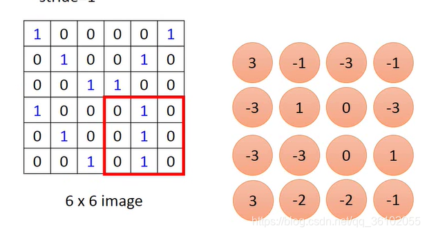
It can be seen that the size of the convolution kernel determines the size of the resulting matrix.
In the process of moving, we move one pixel every time, we can also move multiple pixels at once, that is, adjust the stride to a different value.
Suppose the input pixel matrix is $m\times n$ , the convolution kernel is$a\times b$ , and stride is$s$ then the output matrix size is$(\frac{m-a}{s}+1)\times (\frac{n-b}{s}+1)$。

Multiple channels

For color bitmaps of multiple channels, the convolution kernel we use can no longer be a two-dimensional matrix, but a stack of two-dimensional convolution kernels as many as the number of channels.

For example, the RGB image of three channels, its convolution kernel may be like this,

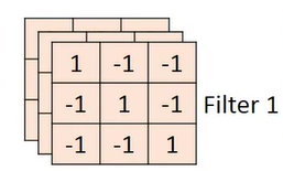
so that the output matrix obtained is also a three-dimensional matrix.
After getting the output, sum the matrix obtained along the dimension of the channel, and then get the final output result.
That is, for a convolution kernel, its final output channel must be 1.

A convolution kernel can scan all areas in the picture to check whether a certain pattern appears. The weight in the convolution kernel is obtained through train.
For a picture, we need to detect more than one specific pattern, so we can use multiple convolution kernels to detect different patterns.

The shape of the output matrix

First of all, there are several parameters that can determine the output shape:

1. Input data $N\times c\times m\times n$
   where N represents the number of samples, and c represents the channel.
2. Convolution kernel size $a\times b$ , and the number of convolution kernels A
3. Stride, padding

Among them, padding is similar to a kind of filling. It will fill a layer of blank pixels in the outer layer of the input matrix to make the original $n\times$The matrix of$m$ becomes$(n+padding\ast 2)\times (m+padding\ast 2)$ The matrix.

With the above parameters, you can get the output matrix shape $N\times A\times m^{\prime }\times n^{\prime }$
其中
$$\begin{gathered} m^{\prime }=\frac{m+padding\ast 2-a}{stride}+1 \\ {n}^{\prime }=\frac{n+padding\ast 2-b}{stride}+1\; It \end{gathered}$$
can be seen that the number of channels of the output matrix is ​​determined by the number of convolution kernels, while m and n are determined by multiple factors.

Pooling

After convolution, the next operation is pooling.
Pooling can also be used as a down-sampling to reduce the scale of features.
There are many kinds of pooling, such as maxpooling, averagepooling, etc. For
example , maxpooling, like convolution, slides to take some areas, and then takes the maximum value of each area as the sample of this area.

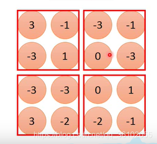
Then stack them together and get the output,

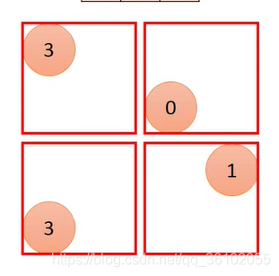
so you get a $2\times 2$ size matrix.
It should be noted that the window is also sliding during the pooling process as in the convolution, so the calculation method of n and m of the output matrix is ​​the same as the above convolution.

After repeated convolution pooling many times, we can get a $N\times c\times n\times$The matrix of$m$ . We straighten it into$N\times (c\ast n\ast m)$ matrix, and then throw it to a fully connected network.

Carefully observe the entire process of CNN, in fact, compared with the ordinary fully connected network, it is an additional process of extracting features through convolution and pooling.

CNN by pytorch

Here, pytorch is used to build a simple CNN network to train the Mnist data set.
First import the necessary packages.

import torch
from torch import nn
from torchvision import transforms
from torchvision import datasets

Then import the data set

compose = transforms.Compose([
    transforms.ToTensor(),
    transforms.Normalize((0.1307,), (0.3081,))
])
batch_size = 600
mnist_train = datasets.MNIST('./datasets/mnist', download=True, train=True, transform=compose)
loader_train = torch.utils.data.DataLoader(dataset=mnist_train, shuffle=True, batch_size=batch_size, num_workers=4)
mnist_test = datasets.MNIST('./datasets/mnist', download=True, train=False, transform=compose)
loader_test = torch.utils.data.DataLoader(dataset=mnist_test, shuffle=True, batch_size=10000)

Next, build the network architecture. The approximate structure is convolution twice, pooling twice, and then put in a fully connected layer with 320 inputs and 10 outputs.
Note that the convolutional layer is actually doing linear operations, so a nonlinear activation function should also be added

class CNN(nn.Module):
    def __init__(self):
        super(CNN, self).__init__()
        self.cv1 = nn.Conv2d(in_channels=1, out_channels=10, kernel_size=5) # 卷积层1
        self.cv2 = nn.Conv2d(in_channels=10, out_channels=20, kernel_size=5) # 卷积层2
        self.maxpooling = nn.MaxPool2d(kernel_size=2) # 池化
        self.liner = nn.Linear(320, 10)
    
    def forward(self, x):
        x = nn.functional.relu(self.cv1(x))
        x = self.maxpooling(x)
        x = nn.functional.relu(self.cv2(x))
        x = self.maxpooling(x)
        x = x.view(x.shape[0], -1)
        x = self.liner(x)
        return x

Then create a model and move it to cuda, create an optimizer, and specify a loss function

moudle = CNN().cuda()
optimizer = torch.optim.SGD(moudle.parameters(), lr=0.1, momentum=0.02)
loss_fun = nn.functional.cross_entropy

Write a function to calculate the acc of the test set

def test():
    with torch.no_grad():
        for batch in loader_test:
            data, target = batch
            data = data.cuda()
            target = target.cuda()
            acc = (torch.argmax(moudle(data), dim=1) == target).sum().item() / target.shape[0]
            print(acc)

Next is the gradient descent part

if __name__ == '__main__':
    for epoch in range(10):
        for i, batch in enumerate(loader_train):
            data, target = batch
            target = torch.LongTensor(target)
            data = data.cuda()
            target = target.cuda()

            y_hat =  moudle(data)
            loss = loss_fun(y_hat, target)

            optimizer.zero_grad()
            loss.backward()
            optimizer.step()
        test()

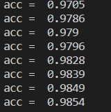
In the end, there is almost an accuracy of 98.5%, and the accuracy will decrease after the calculation, and overfitting will occur.