The data set used here is still CIFAR-10. Since I wrote an article on the classification of the CIFAR data set using AlexNet before, this data set has been introduced in detail. At that time, we directly downloaded the data files of these pictures, and then Use pickle for deserialization to obtain data. For details, please refer to here: Section 16, AlexNet Network Implementation of Convolutional Neural Networks (6)
Similar to MNIST, TensorFlow also has a code file for downloading and importing the CIFAR dataset. The difference is that since TensorFlow 1.0, the Models module inside has been separated, and the code for separating and importing the CIFAR dataset is in the models, so Go to TensorFlow's GitHub website to download it first. Click the download link to start the download .

a description
In this example, a global average pooling layer is used instead of the traditional fully connected layer, a co-convolutional network with 3 convolutional layers is used, the filter is 5x5, and each convolutional layer is followed by a stride of 2x2 The pooling layer, the filter size is 2x2, the last pooling layer is the global average pooling layer, the output is batch_sizex1x1x10, we align the shape transformation to batch_sizex10, get 10 features, and then perform softmax calculation on these 10 features , and the result represents the final classification.
Two import datasets
'''
An introduction to the dataset
'''
batch_size = 128
learning_rate = 1e-4
training_step = 15000
display_step = 200
 #Data set directory
data_dir = ' ./cifar10_data/cifar-10-batches-bin '
print ( ' begin ' )
 #Get training set data
images_train, labels_train = cifar10_input.inputs(eval_data=False,data_dir = data_dir,batch_size= batch_size)
 print ( ' begin data ' )
Note that the cifar10_input.inputs() function is called here. This function is a function to obtain data and returns the corresponding label of the data set. However, this function will crop the image from the original 32x32x3 to 24x24x3. This function uses the test by default. The dataset, if using the training dataset, you can pass the first parameter to eval_data=False. In addition, pass in batch_size and dir, and you can get the batch_size data under dir. We can take a look at the implementation of this function:
def inputs(eval_data, data_dir, batch_size):
  """Construct input for CIFAR evaluation using the Reader ops.

  Args:
    eval_data: bool, indicating if one should use the train or eval data set.
    data_dir: Path to the CIFAR-10 data directory.
    batch_size: Number of images per batch.

  Returns:
    images: Images. 4D tensor of [batch_size, IMAGE_SIZE, IMAGE_SIZE, 3] size.
    labels: Labels. 1D tensor of [batch_size] size.
  """
  if not eval_data:
    filenames = [os.path.join(data_dir, 'data_batch_%d.bin' % i)
                 for i in xrange(1, 6)]
    num_examples_per_epoch = NUM_EXAMPLES_PER_EPOCH_FOR_TRAIN
  else:
    filenames = [os.path.join(data_dir, 'test_batch.bin')]
    num_examples_per_epoch = NUM_EXAMPLES_PER_EPOCH_FOR_EVAL

  for f in filenames:
    if not tf.gfile.Exists(f):
      raise ValueError('Failed to find file: ' + f)

  with tf.name_scope('input'):
    # Create a queue that produces the filenames to read.
    filename_queue = tf.train.string_input_producer(filenames)

    # Read examples from files in the filename queue.
    read_input = read_cifar10(filename_queue)
    reshaped_image = tf.cast(read_input.uint8image, tf.float32)

    height = IMAGE_SIZE
    width = IMAGE_SIZE

    # Image processing for evaluation.
    # Crop the central [height, width] of the image.
    resized_image = tf.image.resize_image_with_crop_or_pad(reshaped_image,
                                                           height, width)

    # Subtract off the mean and divide by the variance of the pixels.
    float_image = tf.image.per_image_standardization(resized_image)

    # Set the shapes of tensors.
    float_image.set_shape([height, width, 3])
    read_input.label.set_shape([1])

    # Ensure that the random shuffling has good mixing properties.
    min_fraction_of_examples_in_queue = 0.4
    min_queue_examples = int(num_examples_per_epoch *
                             min_fraction_of_examples_in_queue)

  # Generate a batch of images and labels by building up a queue of examples.
  return _generate_image_and_label_batch(float_image, read_input.label,
                                         min_queue_examples, batch_size,
                                         shuffle=False)
This function mainly includes the following steps:
- Read the test set filename or the training set filename, and create a filename queue.
- Use a file reader to read the data and labels of an image, and return a class object that holds these tensors of data.
- Crop the image.
- Normalize the input.
- Read batch_size images. (The return is a tensor, which must be executed in the session to get the data)
Three definitions of network structure
'''
Two define the network structure
'''
def weight_variable(shape):
    '''
    Initialize weights

    args:
        shape:权重shape
    '''
    initial = tf.truncated_normal(shape=shape,mean=0.0,stddev=0.1)
    return tf.Variable(initial)

def bias_variable(shape):
    '''
    Initialize bias

    args:
        shape:偏置shape
    '''
    initial =tf.constant(0.1,shape=shape)
    return tf.Variable(initial)


def conv2d(x,W):
    '''
    Convolution operation, after using the SAME padding pooling layer
         out_height = in_hight / strides_height (round up)
         out_width = in_width / strides_width(向上取整)

    args:
        x: The input image shape is [batch,in_height,in_width,in_channels]
        W: Weight shape is [filter_height, filter_width, in_channels, out_channels]
    '''
    return tf.nn.conv2d(x,W,strides=[1,1,1,1],padding='SAME')


def max_pool_2x2(x):
    '''
    The maximum pooling layer, the filter size is 2x2, the 'SAME' padding method after the pooling layer
         out_height = in_hight / strides_height (round up)
         out_width = in_width / strides_width(向上取整)

    args:
        x: The input image shape is [batch,in_height,in_width,in_channels]
    '''
    return tf.nn.max_pool(x,ksize=[1,2,2,1],strides=[1,2,2,1],padding='SAME')


def avg_pool_6x6(x):
    '''
    Global average pooling layer, using a filter of the same size as the original input for pooling, 'SAME' filling method after the pooling layer
         out_height = in_hight / strides_height (round up)
         out_width = in_width / strides_width(向上取整)

    args;
        x: The input image shape is [batch,in_height,in_width,in_channels]
    '''
    return tf.nn.avg_pool(x,ksize=[1,6,6,1],strides=[1,6,6,1],padding='SAME')

def print_op_shape(t):
    '''
    Output the shape of an operation op node
    '''
    print(t.op.name,'',t.get_shape().as_list())


#Define placeholder input_x
= tf.placeholder(dtype=tf.float32,shape=[None,24,24,3])    #image size 24x24x
input_y = tf.placeholder(dtype=tf.float32,shape=[None, 10])         # 0-9 categories

x_image = tf.reshape(input_x,[-1,24,24,3 ])

# 1. Convolutional layer -> Pooling layer
W_conv1 = weight_variable([5,5,3,64 ])
b_conv1 = bias_variable([64])


h_conv1 = tf.nn.relu(conv2d(x_image,W_conv1) + b_conv1) #The     output is [-1,24,24,64]
print_op_shape(h_conv1)
h_pool1 = max_pool_2x2(h_conv1) #The                             output is [-1,12,12,64]
print_op_shape(h_pool1)


# 2. Convolutional layer -> Pooling layer
W_conv2 = weight_variable([5,5,64,64 ])
b_conv2 = bias_variable([64])


h_conv2 = tf.nn.relu(conv2d(h_pool1,W_conv2) + b_conv2) #The     output is [-1,12,12,64]
print_op_shape(h_conv2)
h_pool2 = max_pool_2x2(h_conv2) #The                             output is [-1,6,6,64]
print_op_shape(h_pool2)


# 3. Convolutional layer -> global average pooling layer
W_conv3 = weight_variable([5,5,64,10 ])
b_conv3 = bias_variable([10])

h_conv3 = tf.nn.relu(conv2d(h_pool2,W_conv3) + b_conv3) #The    output is [-1,6,6,10]
print_op_shape(h_conv3)

nt_hpool3 = avg_pool_6x6(h_conv3) #The                          output is [-1,1,1,10]
print_op_shape(nt_hpool3)
nt_hpool3_flat = tf.reshape(nt_hpool3,[-1,10])

y_conv = tf.nn.softmax(nt_hpool3_flat)
Four Definition Solvers
'''
Three Definition Solver
'''

# softmax cross entropy cost function
cost = tf.reduce_mean(-tf.reduce_sum(input_y * tf.log(y_conv),axis=1 ))

#求解器
train = tf.train.AdamOptimizer(learning_rate).minimize(cost)

#Return an accuracy data
correct_prediction = tf.equal(tf.arg_max(y_conv,1),tf.arg_max(input_y,1 ))
 #Accuracy accuracy
= tf.reduce_mean(tf.cast(correct_prediction,dtype=tf. float32))
Five to start the test
'''
Four start training
'' '
sex = tf.Session ();
sess.run(tf.global_variables_initializer())
tf.train.start_queue_runners (sex = sex)

for step in range(training_step):
    image_batch,label_batch = sess.run([images_train,labels_train])
    label_b = np.eye(10,dtype=np.float32)[label_batch]

    train.run(feed_dict={input_x:image_batch,input_y:label_b},session=sess)

    if step % display_step == 0:
        train_accuracy = accuracy.eval(feed_dict={input_x:image_batch,input_y:label_b},session=sess)
        print('Step {0} tranining accuracy {1}'.format(step,train_accuracy))
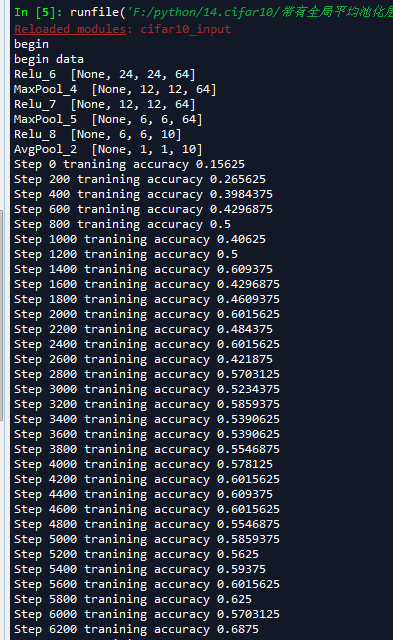
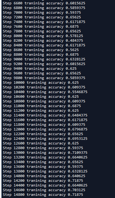
We can see that the accuracy of this model is close to 70%, which is much higher than the 52% accuracy of traditional neural network training in our article in Section 16, AlexNet Network Implementation of Convolutional Neural Networks (6) . And it is a little higher than 60% of AlexNet (AlexNet I iterate less rounds, too because of time-consuming).