The training process of convolutional neural network
The training process of a convolutional neural network is divided into two stages. The first stage is the stage in which data is propagated from low-level to high-level, that is, the forward propagation stage. Another stage is that when the results obtained by forward propagation are inconsistent with expectations, the error is propagated from the high level to the bottom level for training, that is, the back propagation stage. The training process is shown in Figure 4-1. The training process is:
1. The network initializes the weights;
2. The input data is propagated forward through the convolutional layer, the downsampling layer, and the fully connected layer to obtain the output value;
3. Find the error between the output value of the network and the target value;
4. When the error is greater than our expected value, the error is transmitted back to the network, and the errors of the fully connected layer, the downsampling layer, and the convolutional layer are obtained in turn. The error of each layer can be understood as how much the network should bear for the total error of the network; when the error is equal to or less than our expected value, the training ends.
5. Update the weights according to the obtained error. Then go to the second step.

Figure 4-1 The training process of a convolutional neural network
1.1 Forward Propagation Process of Convolutional Neural Networks
In the forward propagation process, the input graphic data is processed by convolution and pooling of multi-layer convolutional layers, and the feature vector is proposed, and the feature vector is passed into the fully connected layer to obtain the result of classification and recognition. When the output result matches our expected value, output the result.
1.1.1 The forward propagation process of the convolutional layer
The forward propagation process of the convolutional layer is that the convolution operation is performed on the input data through the convolution kernel to obtain the convolution operation. For the calculation process of data in the actual network, we take Figure 3-4 as an example to introduce the forward propagation process of the convolutional layer. One of the inputs is a picture of 15 neurons, and the convolution kernel is a 2×2×1 network, that is, the weights of the convolution kernel are W1, W2, W3, W4. Then the convolution process of the convolution kernel for the input data is shown in Figure 4-2 below. The convolution kernel uses a convolution method with a step size of 1 to convolve the entire input image to form a local receptive field, and then perform a convolution algorithm with it, that is, the weight matrix and the eigenvalues of the image are weighted and summed (plus a bias). setting), and then get the output through the activation function.
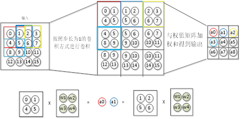
Figure 4-2 The image depth is 1, and the forward propagation process of the convolutional layer
In Figure 3-4, when the image depth is 2, the forward propagation process of the convolutional layer is shown in Figure 4-3. The depth of the input image is 4×4×2, the convolution kernel is 2×2×2, and the forward propagation process is to obtain the weighted sum of the data of the first layer and the weights of the first layer of the convolution kernel, Then, the weighted sum of the data of the second layer and the weights of the second layer of the convolution kernel is obtained, and the weighted sum of the two layers is added to obtain the output of the network.
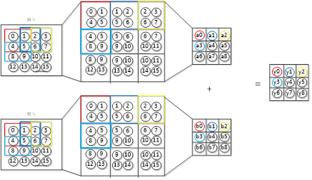
Figure 4-3 The image depth is 2, and the forward propagation process of the convolutional layer
1.1.2 The forward propagation process of the downsampling layer
The features extracted by the upper layer (convolutional layer) are passed as input to the downsampling layer. Through the pooling operation of the downsampling layer, the dimension of the data can be reduced and overfitting can be avoided. Figure 4-4 shows the common pooling methods. The max pooling method is to select the maximum value in the feature map. Mean pooling is to find the average value of the feature map. The random pooling method is to first find the probability of all feature values appearing in the feature map, and then randomly select one of the probabilities as the feature value of the feature map. The higher the probability, the greater the probability of selection.
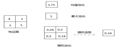
Figure 4-4 Schematic diagram of pooling operation
1.1.3 The forward propagation process of the fully connected layer
After the feature map enters the feature extraction of the convolutional layer and the downsampling layer, the extracted features are passed to the fully connected layer, which is classified through the fully connected layer to obtain a classification model and obtain the final result. Figure 4-5 shows a three-layer fully connected layer. Suppose that in the convolutional neural network, the features of the incoming fully connected layer are x1, x2. Then its forward propagation process in the fully connected layer is shown in Figure 4-5. The first fully connected layer has 3 neurons y1, y2, y3. The weight matrix of these three nodes is W, where b1, b2, and b3 are the offsets of nodes y1, y2, and y3, respectively. It can be seen that in the fully connected layer, the number of parameters = the number of nodes in the fully connected layer × the number of input features + the number of nodes (bias). The forward transfer process is shown in the figure. After the output matrix is obtained, it is activated by the excitation function f(y) and passed to the next layer.
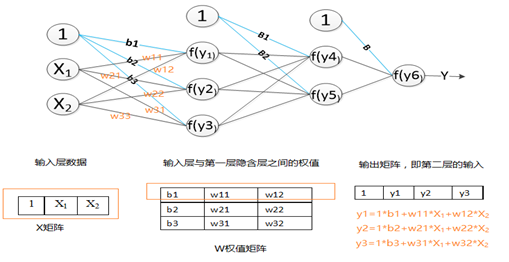
Figure 4-5 The forward propagation process of the fully connected layer
1.2 Backpropagation process of convolutional neural network
When the results of the convolutional neural network output do not match our expectations, the back-propagation process is performed. Find the error between the result and the expected value, then return the error layer by layer, calculate the error of each layer, and then update the weights. The main purpose of this process is to adjust the network weights by training samples and expected values. The error transmission process can be understood in this way. First of all, the data passes through the convolution layer, downsampling layer, and fully connected layer from the input layer to the output layer, and the process of data transmission between layers will inevitably cause data corruption. loss, which leads to errors. The error value caused by each layer is different, so when we find the total error of the network, we need to pass the error into the network to find out how much each layer should take on the total error.
The first step in the training process of backpropagation is to calculate the total error of the network: find the error between the output a(n) of the output layer n and the target value y. The calculation formula is:
 where is the value of the derivative function of the excitation function.
1.2.1 Error transfer between fully connected layers
After the total difference of the network is found, the back-propagation process is carried out, and the error is passed to the upper fully connected layer of the output layer to find out how much error is generated in this layer. The error of the network is caused by the neurons that make up the network, so we require the error of each neuron in the network. To find the error of the previous layer, it is necessary to find out which nodes in the previous layer are connected to the output layer, and then multiply the error by the weight of the node to obtain the error of each node, as shown in the figure:

Figure 4-6 The error propagation process in the fully connected layer
1.2.2 The current layer is a downsampling layer, and the error of the previous layer is calculated
In the downsampling layer, the error is passed to the upper layer according to the pooling method used. If the downsampling layer adopts the max-pooling method, the error is directly passed to the nodes connected to the previous layer. If the mean pooling method is used, the error is evenly distributed to the previous layer of the network. In addition, in the downsampling layer, there is no need to update the weights, and it is only necessary to correctly transfer all the errors to the upper layer.
1.2.3 The current layer is a convolutional layer, and the error of the previous layer is calculated
The convolutional layer adopts the local connection method, which is different from the error transmission method of the fully connected layer. In the convolutional layer, the error transmission is also transmitted by the convolution kernel. In the process of error transmission, we need to find the connection nodes between the convolution layer and the previous layer through the convolution kernel. The process of finding the error of the upper layer of the convolutional layer is as follows: first fill the convolutional layer error with all zeros, then rotate the convolutional layer by 180 degrees, and then use the rotated convolution kernel to convolve Fill the error matrix of the process and get the error of the previous layer. Figure 4-7 shows the error transfer process of the convolutional layer. The upper right of the figure is the forward convolution process of the convolutional layer, and the lower right is the error transfer process of the convolutional layer. As can be seen from the figure, the convolution process of the error is just along the forward propagation process, passing the error to the previous layer.
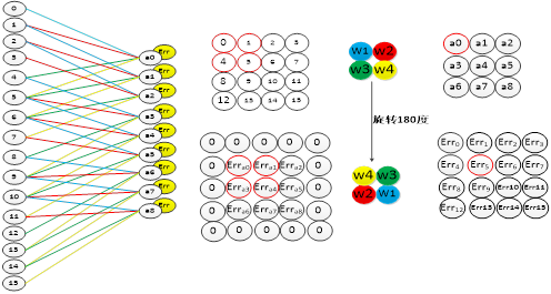
Figure 4-7 The error propagation process of the convolutional layer
1.3 Weight update of convolutional neural network
1.3.1 Weight update of convolutional layer
The error update process of the convolution layer is as follows: the error matrix is used as the convolution kernel, the input feature map is convolved, and the deviation matrix of the weights is obtained, and then the weights of the original convolution kernels are added and updated. After the convolution kernel. As shown in Figure 4-8, it can be seen that the connection of the weights in this convolution method is exactly the same as the connection of the weights in the forward propagation.
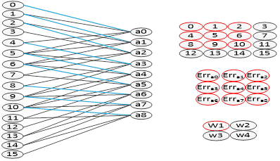
Figure 4-8 The weight update process of the convolution kernel
1.3.2 The weight update process of the fully connected layer
The weight update process in the fully connected layer is:
1. Find the partial derivative value of the weight: the learning rate multiplied by the reciprocal of the excitation function multiplied by the input value;
2. Add the partial derivative to the original weight to obtain a new weight matrix. The specific process is shown in Figure 4-9 (the activation function in the figure is the Sigmoid function).
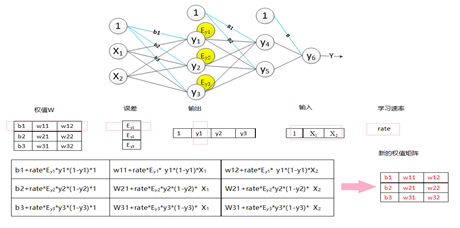
Figure 4-9 The weight update process of the fully connected layer