Policy gradient algorithm (Policy gradient, PG)

Reinforcement learning has three components: actor, environment and reward function,

The actor is our agent, the environment is the opponent, and the reward is the reward given to us by the environment without taking a step. The environment and rewards are beyond our control, but we can adjust the actor's strategy. The actor's strategy determines the actor's action, that is, give Given an input, it outputs the action the actor should now perform.

Policy gradient (Policy gradient, PG)

The strategy is generally recorded as $\pi$ , we generally use the network to represent the strategy, there are some parameters in the network, we use$\theta$ to represent the networkπ \piParameters in$\pi \; .$

If we take the game as an example, the initial screen of the game can be recorded as $s_1$, when the action is executed for the first time $a_1$, the reward after performing the action for the first time is $r_1$Then we entered the second screen, at this time our screen can be recorded as $s_2$, when the action executed for the second time $a_2$, the reward after performing the action for the second time is $r_2$…

When will it end? When the game is over, which means you beat the final boss or you fail midway, it's over.

The following figure can vividly illustrate the above process

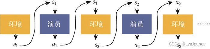
First of all, the environment is a function. This function may be a rule-based model, but we can think of it as a function. This function initially produces a state $s_1$, and then our actor generates the corresponding action $a_1$to the environment, the environment is generated in state $s_2$... this cycle continues until the environment thinks it's over. In a game, we combine the environment and the state to form a trajectory $\tau$
τ = { s 1 , a 1 , s 2 , a 2 , . . . , st , at } \tau = \{s_1,a_1,s_2,a_2,...,s_t,a_t\}t={ s1​,a1​,s2​,a2​,...,st​,at​}
Given the parameters of the actor$\theta$我们可以议出柹发发灦
$$\begin{array}{rl}{p}_{}\left(t\right)& =p(s_1)p_{}(a_1|s_1)p(s_2|s_1,a_1)p_{}(a_2|s_2\left)p\right(s_3|s_2,a_2)...\\ & =p(s_1)\prod _{t=1}^T{p}_{}(a_t|s_t\left)p\right(s_{t+1}|s_t,a_t)\end{array}$$
The probability of a certain trajectory depends on the actions of the environment and the actions of the agent. The action of the environment refers to the action taken by the environment according to the internal parameters of its function or the internal rules. $p(s_{t+1}|s_t,a_t)$ represents the environment, because the environment is set, so usually we cannot control the environment, what can be controlled is$p_{}(a_t|s_t)$ . Given a$s_t$actor to take $a_t$Depends on the actor's parameter $\theta$ So the actions of the agent are controllable by the actor. The actions of the actors are different, and each same trajectory has a different probability of appearance.

A game is called a round, and all the rewards in this game are added up to be called the total reward (total reward), which is the return. We use $R$ to represent it, the actor has to find a way to maximize the rewards that can be obtained, we add up all the rewards of the trajectory to get$R\left(\tau \right)$ represents a certain trajectory$\tau$ 's reward.
$$R\left(\tau \right)=\sum _{t=1}^T{r}_t$$
In a certain game, get $After\; R\left(\tau \right)$ , we wish to adjust the parameter θ \thetainside the actor$\theta$ , such that$R\left(\tau \right)$ The bigger the better, but$R\left(\tau \right)$ is not a scalar, it is a random variable, because the actor may have different output actions even under the same state input, which has a certain degree of randomness. What we can calculate is R ($The\; expected\; value\; of\; R\left(\tau \right)$ , given a certain set of parameters$\theta$ ,$R_{}$The expected value of
$${\bar{R}}_{}=\sum _{t}R\left(\tau \right)p_{}\left(\tau \right)$$
We want to enumerate all possible trajectories$\tau$ , each trajectory has a probability, such asθ \thetaThe model corresponding to$\theta$$\theta$ dies quickly, because this rarely happens, so the trajectory corresponding to this round$The\; probability\; of\; \tau$ is very small, we can according to$\theta$ calculates the probability of a certain trajectory, and then calculates$\tau$ 's total reward. The total reward uses$The\; probability\; of\; \tau$ appearing is weighted, and for all$The\; sum\; of\; \tau$ is the expected value. Given a parameter, we can calculate the expected value as
$${\bar{R}}_{}=\sum _{t}R\left(\tau \right)p_{}\left(t\right)={\mathbb{E}}_{\tau \sim p_{}(t}\left[R\right(\tau )]$$
from the distribution$p_{}\left(\tau \right)$ Sampling a trajectory$\tau$， calculateR$The\; expected\; value\; of\; R\left(\tau \right)$ is the expected reward. We want to maximize the expected reward, and to perform gradient ascent, we first need to calculate the expected reward${\bar{R}}_{}$Variance∇
$$\begin{array}{rl}\nabla {\bar{R}}_{}& =\nabla \sum _{t}R\left(\tau \right)p_{}\left(t\right)\\ & =\sum _{t}R\left(\tau \right)\nabla p_{}(t\end{array}$$
Configuration $p_{}\left(\tau \right)$ from$\theta$ is related, the reward function$R\left(\tau \right)$ does not need to be differentiable, this does not affect us to solve the following problems, here we need to use a formula

Remark1
$$\nabla f(x)=Let\; f\left(x\right)\nabla logf\left(x\right)$$
be a simple random variable in
$$\begin{array}{rl}\nabla {\bar{R}}_{}& =\nabla \sum _{t}R\left(\tau \right)p_{}\left(t\right)\\ & =\sum _{t}R\left(\tau \right)\nabla p_{}\left(t\right)\\ & =\sum _{t}R\left(\tau \right)p_{}\left(\tau \right)\nabla logp{}_{}\left(t\right)\\ & ={\mathbb{E}}_{\tau \sim p_{}(t}\left[R\right(\tau )\nabla logp{}_{}(t)\end{array}$$
The actual expected value cannot be calculated, so we sample N $\tau$ and calculate each value, adding up each value, you can get the gradient.
$$\begin{array}{rl}\nabla {\bar{R}}_{}& \approx \frac{1}{N}\sum _{n=1}^{N}R(t^n)\nabla log{p}_{}(t^n)\\ & =\frac{1}{N}\sum _{n=1}^{N}R(t^n)\nabla \left(logp(s_1)+\sum _{t=1}^{T}log{p}_{}(a_t|s_t)+\sum _{t=1}^{T}logp{}_{(}{s}_{t+1}|a_t,s_t)\right)\\ & =\frac{1}{N}\sum _{n=1}^{N}R\left(t^n\right)\left(\nabla logp(s_1)+\nabla \sum _{t=1}^{T}logp{}_{}(a_t|s_t)+\nabla \sum _{t=1}^{T}logp{}_{(}{s}_{t+1}|a_t,s_t)\right)\\ & =\frac{1}{N}\sum _{n=1}^{N}R\left(t^n\right)\left(\nabla \sum _{t=1}^{T}logp{}_{}(a_t|s_t)\right)\\ & =\frac{1}{N}\sum _{n=1}^{N}R\left(t^n\right)\left(\sum _{t=1}^T\nabla log{p}_{}(a_t|s_t)\right)\\ & =\frac{1}{N}\sum _{t=1}^T\sum _{n=1}^{N}R(t^n)\nabla log{p}_{}(a_t^n|s_t^n)\end{array}$$
There are two terms above $\nabla logp(s_1)$ and $\sum_{t=1}^{T}log \ p_(s_{t+1}|a_t,s_t) $ are gone directly, here we need to explain, because we are here to find the gradient for the agent Find the gradient of the parameter, that is, for$\theta$ finds the gradient, both values ​​come from the environment, or it can be said that$\theta$ , so their gradient is 0.

We can intuitively understand the equation we derived above, that is, during the sampling process, we sampled a pair of data $(s_t,a_t)$ , if our entire trajectory$The\; final\; reward\; sum\; of\; \tau$ is positive, then we need to strengthen the state$s_t$take action $a_t$probability, otherwise we have to reduce this probability.

We have calculated the gradient, and the next step is to update our network with this gradient using the gradient ascent method.

let's go into a little more detail

We will collect n trajectories respectively $t^1,t^2,...,t^n$ , these n trajectories contain some state pairs, for example, the first trajectory contains state pairs$\{(s_1^1,a_1^1),(s_2^1,a_2^1),...,(s_{m_1}^1,a_{m_1}^1,\}$ , the second trajectory contains state pairs$\{(s_1^2,a_1^2),(s_2^2,a_2^2),...,(s_{m_2}^2,a_{m_2}^2,\}$ , and their rewards are$R(t^1),R(t^2),...,R\left(t^n\right)$At this time, we can bring the sampled data into the formula to calculate the gradient, that is, each$s$ and$Take\; out\; a$ , calculate the logarithmic probability of taking a certain action in a certain state, multiply the probability by a weight (that is, the reward of this game), and update the model after calculating the gradient.

After updating the model, resample the data and update the model. Note that the general **policy gradient (PG)** sampled data will only be used once. We sample this data, then use this data to update parameters, and then discard this data. Then resample the data to update the parameters.

Policy Gradient Optimization Strategy

Add a baseline

Take an action in a given state, if the reward for this action is positive, we need to encourage this behavior and increase the probability, if the reward for this action is negative, we need to reduce the probability, but some The rewards obtained in the game are all positive, the reward for taking certain actions is 0, and the reward for taking certain actions is 20.

Suppose we have three actions a, b, c, we want to increase the probability of these three actions, but their front weight $R\left(\tau \right)$ is different. The weights vary from big to small. If the weight is small, the probability of the action will increase less; if the weight is large, the probability of the action will increase more, because the logarithmic probability is also a probability. In the end, it still passes through a softmax layer for output, so even if the probability of a is the highest among the three actions, but after all the probabilities are added, if more b is added, b may become the output with the highest probability.

[External link picture transfer failed, the source site may have an anti-leeching mechanism, it is recommended to save the picture and upload it directly (img-4JCkKCGA-1680158181247) (C:\Users\LoveSS\Desktop\Enhanced Learning.picture\NeatReader-1679022396646.png )]

This is an ideal situation. The problem is that we are only doing sampling. Some actions may not be sampled. Suppose we sampled b, but c did not sample a. Now all rewards are positive, and the probability of all actions will be increased. , but a has not been sampled, so a has no reward, then his probability can only decrease, which is unreasonable, so we expect our reward to be positive or negative

We can modify the above formula and add a baseline
$$\nabla {\bar{R}}_{}\approx \frac{1}{N}\sum _{t=1}^T\sum _{n=1}^N\left(R\right(t^n)-b)\nabla log{p}_{}(a_t^n|s_t^n)$$
where $b$ is called the baseline. In this way,$R\left(t^n\right)-The\; term\; b$ can be positive or negative.

assign appropriate points

Assign appropriate credits to each action, as long as they are in the same round and in the same game, all state-action pairs are weighted with the same reward item. This is obviously unfair, because in the same game, some actions may be good and some actions may be bad. Assuming that the outcome of the entire game is good, it does not mean that every action in the game is good. If the result of the whole game is bad, it does not mean that every action in the game is bad. So we hope that we can multiply different weights in front of each different action. The different weights of each action reflect whether each action is good or bad.

One way is to calculate the reward of a certain state-action pair, instead of adding up all the rewards obtained in the entire game, only calculate the reward obtained after the execution of this action. Because what happened in this game before performing this action has nothing to do with performing this action, so the rewards obtained before performing this action cannot be regarded as the contribution of this action. We add up all the rewards that occur after performing this action, which is the real contribution of this action.

The original weight is the sum of the rewards of the whole game, now it is changed from a certain moment $t$ starts, assuming the action is at$t$ started execution, from$tThe$ sum of all rewards until the end of the game can represent the quality of this action.

Going one step further, we discount the future rewards, that is,
$$\nabla {\bar{R}}_{}\approx \frac{1}{N}\sum _{t=1}^T\sum _{n=1}^N(\sum _{t^{\prime }=t}^{T_n}{c}^{t^{\prime }-t}{r}_{t^{\prime }}^n-b)\nabla log{p}_{}(a_t^n|s_t^n)$$
Why make a discount on future rewards? Because although at a certain moment, the execution of a certain action will affect all the subsequent results (it is possible that the action performed at a certain moment, the next reward is the credit of this action), but in general, The longer the delay, the less impact the action has.

$b$ can be made dependent, in fact$b$ is usually estimated by a network, it is the output of a network, we put$R-The\; term\; b$ is called the advantage function (advantage function), using$A^i(s_t,a_t)$ to represent the advantage function, which depends on$s$和$a$ , we just want to calculate the value of the advantage function when taking a certain action in a certain state. When calculating the value of the advantage function, we need a model to interact with the environment, so that we can know the reward sum to be obtained next. The significance of the advantage function lies in The advantages of taking a certain action in a certain state compared to other actions, the advantage function is not absolutely good, but relatively good, that is, relative advantage (relative advantage), because in the advantage function we will subtract the baseline$b$ , so this action is relatively good but not absolutely good,$A^i(s_t,a_t)$ can usually be estimated by a network called Critic

Monte Carlo policy gradient (REINFORCE)

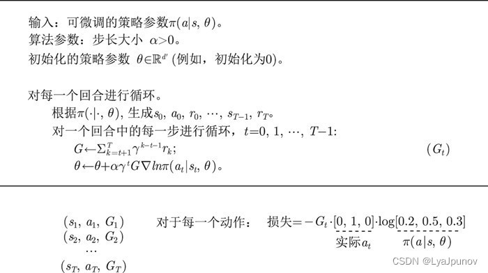
Let’s introduce REINFORCE, the most classic algorithm in policy gradient. REINFORCE uses the round update method. In terms of code processing, it first obtains the reward of each step, and then calculates the future total reward G t G_t of each step $G_t$, each $G_t$代入
$$\nabla {\bar{R}}_{}\approx \frac{1}{N}\sum _{t=1}^T\sum _{n=1}^N{G}_t\nabla log{\pi }_{}(a_t^n|s_t^n)$$
Optimize the output of each action. So when we write code, we will design a function. The input of this function is the reward obtained at each step, and the output is the future total reward of each step. Because the future total reward can be written as
$$\begin{array}{rl}{G}_t& =\sum _{k=t+1}^T{c}^{k-t-1}{r}_k\\ & =r_{t-1}+c{G}_{t-1}\end{array}$$
The Monte Carlo policy gradient calculates the gradient for each action $\nabla ln\pi (a_t|s_t,\theta )$ , when calculating the code, we need to obtain the output of the neural network, the neural network will output the probability value corresponding to each action, and then we can obtain the actual action$a_t$, convert the action into one-hot encoding, such as ([0,1,0]), and multiply it with the logarithm of the output probability [0.1,0.2,0.7] to get $ln\pi (a_t|s_t,i)$

Algorithm process

the code

We give code examples here

import torch as t
import numpy as np
import gym
import torch.optim as optim
import torch.nn as nn
import torch.nn.functional as F

gamma = 0.95  # 折扣因子
render = False  # 是否显示画面
lr = 0.001  # 学习率

env = gym.make("CartPole-v1")

class PGModule(nn.Module):
    def __init__(self, n_input, n_output) -> None:
        super(PGModule, self).__init__()
        self.net = nn.Sequential(
            nn.Linear(n_input, 128),
            nn.ReLU(),
            nn.Linear(128, 64),
            nn.ReLU(),
            nn.Linear(64, n_output),
        )

        self.optimizer = optim.Adam(self.net.parameters(), lr=lr)

        self.episode_s = []
        self.episode_a = []
        self.episode_r = []

    def store(self, state, action, reward):  # 保留回合中的数据
        self.episode_s.append(state)
        self.episode_a.append(action)
        self.episode_r.append(reward)

    def forward(self, input):
        return F.softmax(self.net(input), dim=1)

    def clear(self):
        self.episode_s = []
        self.episode_a = []
        self.episode_r = []

    def learn(self):
        G = []
        g = 0
        for r in self.episode_r[::-1]:
            g = gamma * g + r
            G.insert(0, g)
        for i, s in enumerate(self.episode_s):
            state = t.unsqueeze(t.tensor(s, dtype=t.float), dim=0)
            a = self.episode_a[i]
            a_prob = self.forward(state).flatten()  # 展开
            g = G[i]
            loss = - g * t.log(a_prob[a])
            self.optimizer.zero_grad()
            loss.backward()
            self.optimizer.step()


class trainModule():
    def __init__(self):
        self.net = PGModule(4, 2)

    def choose_action(self, observation) -> None:
        observation_tensor_unsqueeze = t.unsqueeze(t.FloatTensor(observation), 0)
        output = self.net.forward(observation_tensor_unsqueeze)
        action = np.random.choice(range(output.detach().numpy().shape[1]), p=output.squeeze(dim=0).detach().numpy())
        return action

    def get_once(self) -> None:
        for j in range(400):
            observation, info = env.reset(seed=42)
            allreward = 0
            while True:
                action = self.choose_action(observation)
                observation_, reward, terminated, truncated, info = env.step(action)
                self.net.store(observation, action, reward)
                observation = observation_
                allreward += reward
                if render:
                    env.render()
                if terminated or truncated:
                    self.net.learn()
                    self.net.clear()
                    print(f"j = {
      
      j}  reward is {
      
      allreward}")
                    break

T = trainModule()
T.get_once()

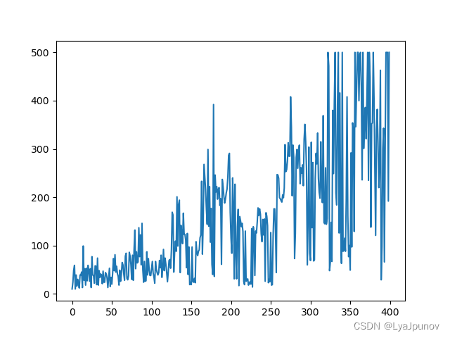
There is one thing to note here. At first I thought there was something wrong with my code, but later I found out that someone else wrote it in the same way. After changing the parameters, it can converge to more than 200 and 300. It is not stable yet. The highest score of the game "CartPole-v1" is 500, this method is still a bit old and not very useful anymore.

Then I slightly expanded the network scale and adopted the game "CartPole-v0". It is a bit of a problem to see this curve anyway.

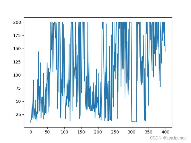
Adjusted the parameters again

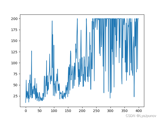
Change the game "CartPole-v1", the result is not bad, I can only say that it is better than horrible