1 Introduction to Policy Gradient
1.1 Policy-based and value-based reinforcement learning methods are different
Reinforcement learning is a mechanism for learning correct behavior through rewards and punishments. There are many different members in the family. They have learning rewards and punishments, and choose behaviors based on what they think are high values, such as Q-Learning, Deep-Q-network. There are also methods that directly output behaviors without analyzing rewards and punishments. This is The Policy Gradient we are going to talk about today adds a neural network to output predicted actions. Compared with value-based methods, the biggest advantage of Policy Gradient's direct output of actions is that it can select actions in a continuous interval, while value-based methods, such as Q-Learning, if it calculates the value of an infinite number of actions, So he chooses to behave, which is too much for him.
1.2 Algorithm update
It is certainly convenient to have a neural network, but how do we reverse the error transfer of the neural network? What is the error of Policy Gradient? The answer is no error. But he is indeed carrying out a kind of backward transmission. The purpose of this back pass is to make the selected behavior more likely to happen next time. But how do we determine whether this behavior should increase the probability of being selected? At this time, reward rewards and punishments can come in handy at this time.
1.3 Specific update steps
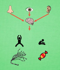
Now demonstrate again, the observed information is analyzed by the neural network, and the behavior on the left is selected, and we directly carry out the reverse transmission, so that the possibility of being selected next time increases, but the reward and punishment information tells us that this behavior is not correct. Okay, so the increase in our action possibilities is reduced accordingly. In this way, rewards can be used to control the backward pass of our neural network. Let’s take another example. If the observation information this time makes the neural network choose the behavior on the right, and then the behavior on the right wants to be transmitted in reverse, so that the behavior on the right will be selected a little more next time. At this time, the reward and punishment information will also Come, tell us that this is a good behavior, then we will increase our efforts in this reverse pass, so that he will be selected more violently next time. This is the core idea of Policy Gradient.
2 Policy Gradient algorithm update
The free download address of all codes is as follows:
https://download.csdn.net/download/shoppingend/85194070
2.1 Main points
Policy Gradient is a big family in RL. It is not like the Value-based method (Q-Learning, Sarsa), but it also receives environmental information (observation). The difference is that it does not output the value of the action, but the specific That action, so that the Policy Gradient skips the value stage. And one of the biggest advantages of Policy Gradient is that the action output can be a continuous value. The value-based method we mentioned before outputs discontinuous values, and then the action with the largest value is selected. The Policy Gradient can select an action on a continuous distribution.
2.2 Algorithm
The simplest Policy Gradient algorithm we introduce is an update based on the entire round of data, also called the REINFORCE method. This method is the most basic method of Policy Gradient. With this foundation, we will do more advanced ones.
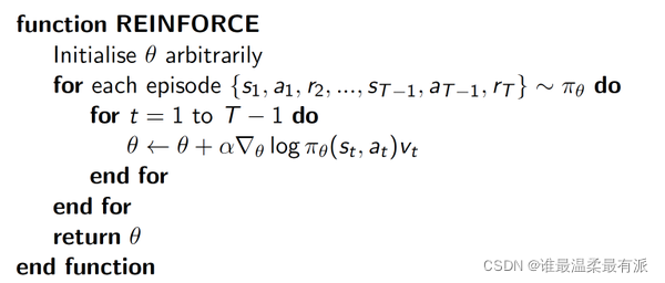
Δ(log(Policy(s,a))*V represents the surprise degree of the selected action a in state s, if the probability of Policy(s,a) is smaller, the reverse log(Policy(s,a))( That is, -log§) is bigger. If you get a large R when Policy(s,a) is small, that is, a large V, then -Δ(log(Policy(s,a))* The V is bigger, which means more surprised, (I chose an action that is not often selected, but found that it can get a good reward, so I have to make a major modification to my parameters this time). This is The physical meaning of astonishment is gone.
2.3 Algorithm code formation
First define the loop for the main update:
import gym
from RL_brain import PolicyGradient
import matplotlib.pyplot as plt

RENDER = False  # 在屏幕上显示模拟窗口会拖慢运行速度, 我们等计算机学得差不多了再显示模拟
DISPLAY_REWARD_THRESHOLD = 400  # 当 回合总 reward 大于 400 时显示模拟窗口

env = gym.make('CartPole-v0')   # CartPole 这个模拟
env = env.unwrapped     # 取消限制
env.seed(1)     # 普通的 Policy gradient 方法, 使得回合的 variance 比较大, 所以我们选了一个好点的随机种子

print(env.action_space)     # 显示可用 action
print(env.observation_space)    # 显示可用 state 的 observation
print(env.observation_space.high)   # 显示 observation 最高值
print(env.observation_space.low)    # 显示 observation 最低值

# 定义
RL = PolicyGradient(
    n_actions=env.action_space.n,
    n_features=env.observation_space.shape[0],
    learning_rate=0.02,
    reward_decay=0.99,   # gamma
    # output_graph=True,    # 输出 tensorboard 文件
)
main loop:
for i_episode in range(3000):

    observation = env.reset()

    while True:
        if RENDER: env.render()

        action = RL.choose_action(observation)

        observation_, reward, done, info = env.step(action)

        RL.store_transition(observation, action, reward)    # 存储这一回合的 transition

        if done:
            ep_rs_sum = sum(RL.ep_rs)

            if 'running_reward' not in globals():
                running_reward = ep_rs_sum
            else:
                running_reward = running_reward * 0.99 + ep_rs_sum * 0.01
            if running_reward > DISPLAY_REWARD_THRESHOLD: RENDER = True     # 判断是否显示模拟
            print("episode:", i_episode, "  reward:", int(running_reward))

            vt = RL.learn() # 学习, 输出 vt, 我们下节课讲这个 vt 的作用

            if i_episode == 0:
                plt.plot(vt)    # plot 这个回合的 vt
                plt.xlabel('episode steps')
                plt.ylabel('normalized state-action value')
                plt.show()
            break

        observation = observation_
3 Policy Gradient thinking decision
3.1 Main code structure
Using the basic Policy gradient algorithm, it looks very similar to the previous value-based algorithm.
class PolicyGradient:
    # 初始化 (有改变)
    def __init__(self, n_actions, n_features, learning_rate=0.01, reward_decay=0.95, output_graph=False):

    # 建立 policy gradient 神经网络 (有改变)
    def _build_net(self):

    # 选行为 (有改变)
    def choose_action(self, observation):

    # 存储回合 transition (有改变)
    def store_transition(self, s, a, r):

    # 学习更新参数 (有改变)
    def learn(self, s, a, r, s_):

    # 衰减回合的 reward (新内容)
    def _discount_and_norm_rewards(self):
initialization:
class PolicyGradient:
    def __init__(self, n_actions, n_features, learning_rate=0.01, reward_decay=0.95, output_graph=False):
        self.n_actions = n_actions
        self.n_features = n_features
        self.lr = learning_rate     # 学习率
        self.gamma = reward_decay   # reward 递减率

        self.ep_obs, self.ep_as, self.ep_rs = [], [], []    # 这是我们存储 回合信息的 list

        self._build_net()   # 建立 policy 神经网络

        self.sess = tf.Session()

        if output_graph:    # 是否输出 tensorboard 文件
            # $ tensorboard --logdir=logs
            # http://0.0.0.0:6006/
            # tf.train.SummaryWriter soon be deprecated, use following
            tf.summary.FileWriter("logs/", self.sess.graph)

        self.sess.run(tf.global_variables_initializer())
3.2 Establish Policy Neural Network
The neural network we are going to build this time is like this:
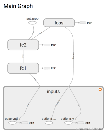
because this is reinforcement learning, there is no y label in the supervised learning in the neural network. Instead, we choose the action.
class PolicyGradient:
    def __init__(self, n_actions, n_features, learning_rate=0.01, reward_decay=0.95, output_graph=False):
        ...
    def _build_net(self):
        with tf.name_scope('inputs'):
            self.tf_obs = tf.placeholder(tf.float32, [None, self.n_features], name="observations")  # 接收 observation
            self.tf_acts = tf.placeholder(tf.int32, [None, ], name="actions_num")   # 接收我们在这个回合中选过的 actions
            self.tf_vt = tf.placeholder(tf.float32, [None, ], name="actions_value") # 接收每个 state-action 所对应的 value (通过 reward 计算)

        # fc1
        layer = tf.layers.dense(
            inputs=self.tf_obs,
            units=10,   # 输出个数
            activation=tf.nn.tanh,  # 激励函数
            kernel_initializer=tf.random_normal_initializer(mean=0, stddev=0.3),
            bias_initializer=tf.constant_initializer(0.1),
            name='fc1'
        )
        # fc2
        all_act = tf.layers.dense(
            inputs=layer,
            units=self.n_actions,   # 输出个数
            activation=None,    # 之后再加 Softmax
            kernel_initializer=tf.random_normal_initializer(mean=0, stddev=0.3),
            bias_initializer=tf.constant_initializer(0.1),
            name='fc2'
        )

        self.all_act_prob = tf.nn.softmax(all_act, name='act_prob')  # 激励函数 softmax 出概率

        with tf.name_scope('loss'):
            # 最大化 总体 reward (log_p * R) 就是在最小化 -(log_p * R), 而 tf 的功能里只有最小化 loss
            neg_log_prob = tf.nn.sparse_softmax_cross_entropy_with_logits(logits=all_act, labels=self.tf_acts) # 所选 action 的概率 -log 值
            # 下面的方式是一样的:
            # neg_log_prob = tf.reduce_sum(-tf.log(self.all_act_prob)*tf.one_hot(self.tf_acts, self.n_actions), axis=1)
            loss = tf.reduce_mean(neg_log_prob * self.tf_vt)  # (vt = 本reward + 衰减的未来reward) 引导参数的梯度下降

        with tf.name_scope('train'):
            self.train_op = tf.train.AdamOptimizer(self.lr).minimize(loss)
Why use loss=-log(prob)*Vt as loss. To put it simply, two types of lines are mentioned above to calculate neg_log_prob. These two types of lines are exactly the same, except that the second one is the expansion of the first one. If you look closely at the first row, it is cross-entropy in the neural network classification problem. The parameters of the neural network are improved according to this ground truth using softmax. This is obviously not much different from a classification problem. We can understand this neg_log_prob as a cross-entropy classification error. The label in the classification problem is the y corresponding to the real x, and in our Policy Gradient, x is the state, and y is the action number it does according to this x. So it can also be understood that the action it does according to x is always correct (the action it comes out is always the correct label, and he will always modify his parameters according to this correct label. But this is not the case, his actions are not necessarily all It is the correct label, which is the difference between Policy Gradient and classification.
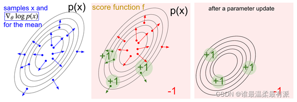
In order to ensure that this action is the correct label, our loss is multiplied by Vt on the original cross-entropy line, and Vt is used to tell the cross Is the gradient calculated by -entropy a trustworthy gradient. If Vt is small or negative, it means that the gradient descent is in the wrong direction, and we should update the parameters in another direction. If this Vt is positive, or If it is very large, Vt will praise the gradient from cross-entropy, and the gradient will drop in this direction. There is a picture below, which is exactly the idea explained.
And why is loss=-log(prob) Vt instead of loss= -prob Vt. The reason is that the prob here comes from softmax, and the calculation of all parameter gradients in the neural network uses cross-entropy, and then multiplies this gradient by Vt to control the direction and intensity of gradient descent.
3.3 Selection behavior
This behavior is no longer selected by Q-value, but by probability. Even without epsilon-greedy, it has a certain degree of randomness.
class PolicyGradient:
    def __init__(self, n_actions, n_features, learning_rate=0.01, reward_decay=0.95, output_graph=False):
        ...
    def _build_net(self):
        ...
    def choose_action(self, observation):
        prob_weights = self.sess.run(self.all_act_prob, feed_dict={

    self.tf_obs: observation[np.newaxis, :]})    # 所有 action 的概率
        action = np.random.choice(range(prob_weights.shape[1]), p=prob_weights.ravel())  # 根据概率来选 action
        return action
3.4 Storage round
This part is to add the observation, action, and reward of this step to the list. Because the list needs to be cleared after the end of this round, and then the data for the next round will be stored, so we will clear the list in learn()
class PolicyGradient:
    def __init__(self, n_actions, n_features, learning_rate=0.01, reward_decay=0.95, output_graph=False):
        ...
    def _build_net(self):
        ...
    def choose_action(self, observation):
        ...
    def store_transition(self, s, a, r):
        self.ep_obs.append(s)
        self.ep_as.append(a)
        self.ep_rs.append(r)
3.5 Learning
The learn() in this section is very simple. First of all, we have to manipulate all the reawrds in this round to make it more suitable for learning. The first is to use γ to attenuate future rewards as time progresses, and then to reduce the Policy Gradient round variance to a certain extent.
class PolicyGradient:
    def __init__(self, n_actions, n_features, learning_rate=0.01, reward_decay=0.95, output_graph=False):
        ...
    def _build_net(self):
        ...
    def choose_action(self, observation):
        ...
    def store_transition(self, s, a, r):
        ...
    def learn(self):
        # 衰减, 并标准化这回合的 reward
        discounted_ep_rs_norm = self._discount_and_norm_rewards()   # 功能再面

        # train on episode
        self.sess.run(self.train_op, feed_dict={


             self.tf_obs: np.vstack(self.ep_obs),  # shape=[None, n_obs]
             self.tf_acts: np.array(self.ep_as),  # shape=[None, ]
             self.tf_vt: discounted_ep_rs_norm,  # shape=[None, ]
        })

        self.ep_obs, self.ep_as, self.ep_rs = [], [], []    # 清空回合 data
        return discounted_ep_rs_norm    # 返回这一回合的 state-action value
Look at discounted_ep_rs_norm again
vt = RL.learn() # 学习, 输出 vt, 我们下节课讲这个 vt 的作用

if i_episode == 0:
    plt.plot(vt)    # plot 这个回合的 vt
    plt.xlabel('episode steps')
    plt.ylabel('normalized state-action value')
    plt.show()
Finally, how to use the algorithm to realize the attenuation of future rewards
class PolicyGradient:
    def __init__(self, n_actions, n_features, learning_rate=0.01, reward_decay=0.95, output_graph=False):
        ...
    def _build_net(self):
        ...
    def choose_action(self, observation):
        ...
    def store_transition(self, s, a, r):
        ...
    def learn(self):
        ...
    def _discount_and_norm_rewards(self):
        # discount episode rewards
        discounted_ep_rs = np.zeros_like(self.ep_rs)
        running_add = 0
        for t in reversed(range(0, len(self.ep_rs))):
            running_add = running_add * self.gamma + self.ep_rs[t]
            discounted_ep_rs[t] = running_add

        # normalize episode rewards
        discounted_ep_rs -= np.mean(discounted_ep_rs)
        discounted_ep_rs /= np.std(discounted_ep_rs)
        return discounted_ep_rs
Article source: Mofan Reinforcement Learning https://mofanpy.com/tutorials/machine-learning/reinforcement-learning/