This article introduces the method of reading Excel table file data and drawing histograms and bar charts with multiple series based on packages and packages in R language.readxlggplot2
First, let's configure the R language readxlpackages and packages we need ggplot2; among them, readxlthe package is used to read the data of the Excel table file, and ggplot2the package is used to draw the histogram. The method of downloading the package is also very simple. Taking readxlthe package as an example, we can enter the following code.
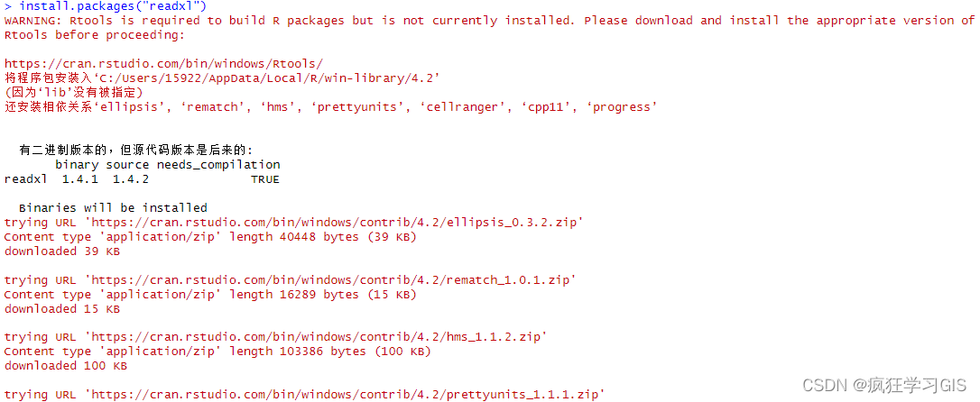
install.packages("readxl")
After entering the code, press 回车the key to run the code; as shown in the figure below.
After readxlthe package download is complete, configure the package in the same way ggplot2.
install.packages("ggplot2")
In addition, when using code for data analysis and visualization, sometimes it is necessary to convert long data and wide data to the data (the specific meaning will be introduced later), here we need to use another R language package reshape2, and we are here Configure them together.
install.packages("reshape2")
Next, we can start writing code. First, we import the packages we need.
library(readxl)
library(ggplot2)
library(reshape2)
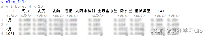
Then, we read the data of the Excel table file; here we use the functions readxlin the package read_excel()to read the table data. Among them, the first parameter of the function indicates the path and name of the Excel table file to be read, and the second parameter indicates which Sheet the data is in; since the data I need here is stored in the first Sheet of the Excel file , so just choose.2sheet = 2
xlsx_file <- read_excel(r"(E:\02_Project\01_Chlorophyll\ClimateZone\Split\Result\Result.xlsx)", sheet = 2)
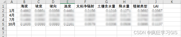
Where, originally in the table file my data looks like this.
Through the above code, we can read the data into the R language; the specific format is shown in the figure below. It can be seen that the read-in data is a tibblecategory variable, tibblewhich is an improvement of Data Frame format data, and here we can treat it as Data Frame format data for subsequent processing.
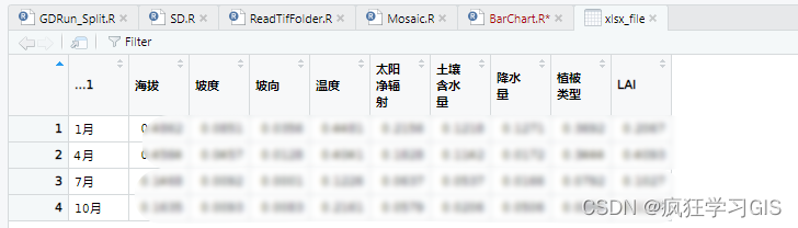
In addition, if you use RStudio software to write code, you can also double-click this variable to see what the read-in data looks like more intuitively, as shown in the figure below.
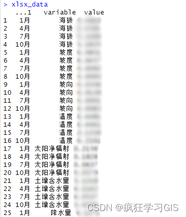
Next, we need to convert the length and width of the data. First of all, in simple terms, wide data is the data shown in the figure above, and long data is the data shown in the figure below; among them, when we obtain and record original data, we often obtain wide data , because this One type of data is more intuitive and easier to record; when data analysis software or codes are used for in-depth processing or visualization of data, the system often needs long data . Therefore, we need to convert wide data and long datamelt() here; this conversion can be realized through functions, and the specific code is as follows.
xlsx_data <- melt(xlsx_file, id.var = "...1")
Among them, melt()the first parameter of the function indicates the variable that needs to be converted, and the second parameter is the ID variable , which is generally the first column of data that expresses the serial number of the data ; I am here because there is no serial number in the original Excel data That column of data, so the first column of the original data is selected as the ID variable . After executing the above code, the long data we get is shown in the figure below.
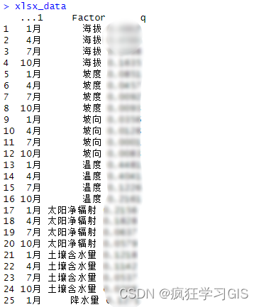
In addition, melt()when the function is running, you can also specify the column name after data conversion. As shown in the following code, we want to set the name of the column representing the variable to Factor, and set the name of the column representing the observed value to q.
xlsx_data <- melt(xlsx_file, id.var = "...1", variable.name = "Factor", value.name = "q")
Execute the above code, and the obtained long data is shown in the figure below.
Of course, it needs to be mentioned here that the conversion of wide data and long data involves a lot of content; if you need it, you can check melt()the official help document of the function.
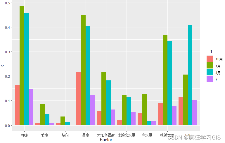
Once the data format conversion is complete, we can start plotting. Here we can draw the histogram directly through the functions ggplot2of the package ggplot(); the specific code is as follows.
ggplot(data = xlsx_data, mapping = aes(x = Factor, y = q, fill = ...1)) + geom_bar(stat = "identity", position = "dodge")
Among them, ggplot()the first parameter of the function dataindicates the data that needs to participate in the drawing, and the second parameter mappingindicates which column of data we need to use as the X axis and which column as the Y axis; at the same time, its internal fillparameters indicate that we need to divide the histogram into Multiple series (if your histogram has only 1one series, then fillthis parameter is not needed), and the variable specified later means that we need to distinguish the series of data based on this variable. Next, the parameters after the plus sign geom_barare what we need to set to draw a multi-series histogram, where positionthe parameter is set to "dodge"indicate that we want to place different series in parallel (if positionthe parameter is not set, the columns of different series will be vertical Stacked, sort of like a stacked histogram ).
Execute the above code to get the following result.
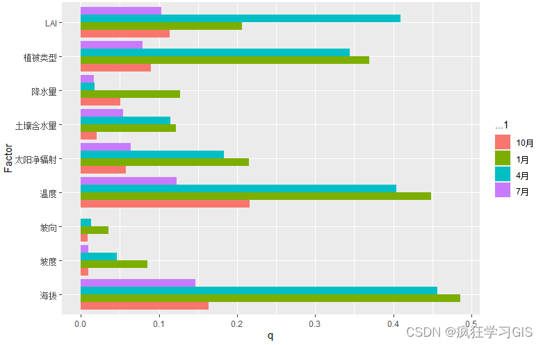
In addition, if you want the histogram to stretch horizontally, just add + coord_flip()the code at the end.
ggplot(data = xlsx_data, mapping = aes(x = Factor, y = q, fill = ...1)) + geom_bar(stat = "identity", position = "dodge") + coord_flip()
Execute the above code to get the following result.
Here, we just ggplot()made a preliminary introduction to the function; for a more in-depth understanding of it, you can directly check its official help document.
So far, you're done.
Welcome to pay attention: Crazy learning GIS