#Foreword
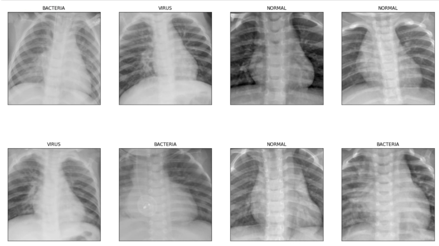
Based on convolutional neural network pneumonia picture recognition and classification, the picture is an X-ray lung map, and the recognition and classification are required to be classified into three categories "normal (NORMAL), bacterial pneumonia (BACTERIA), viral pneumonia (VIRUS)", which can be calculated. The classification accuracy rate, and the image recognition accuracy rate is at least 80%, and the data set is divided into "training group, test group, and verification group".
1. Effect demonstration
2. Video demonstration
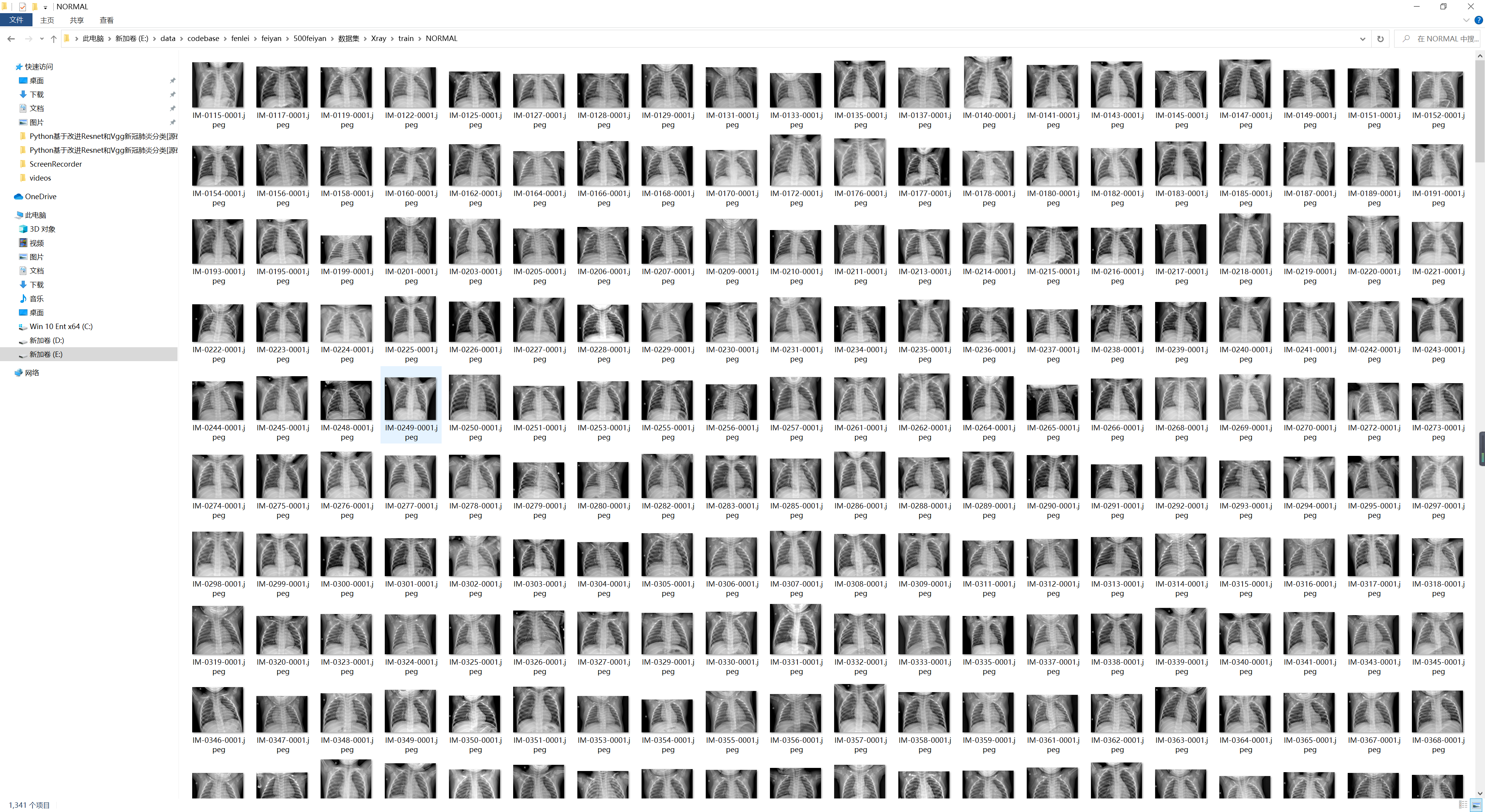
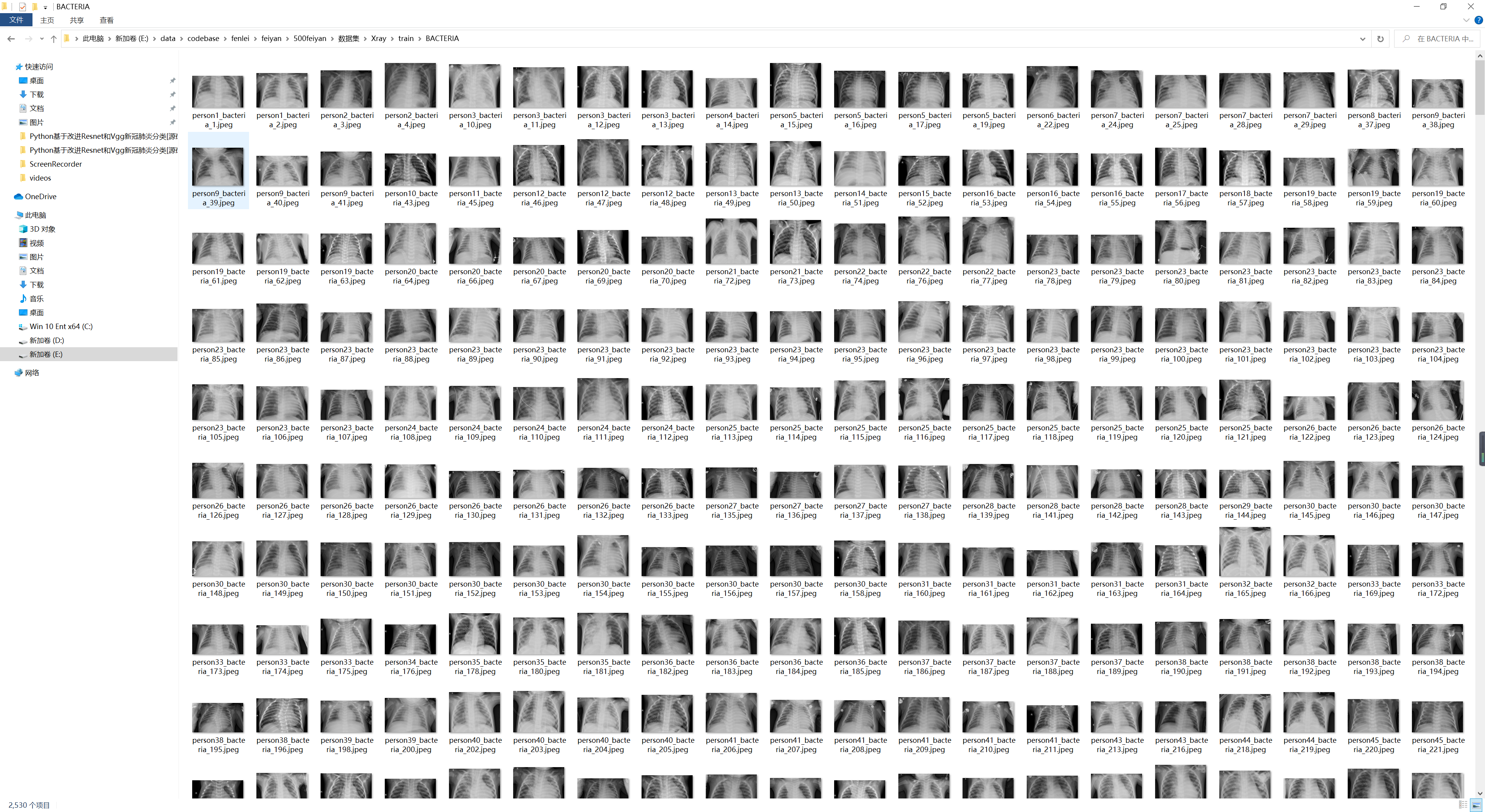
3. Collection of datasets
normal (NORMAL)
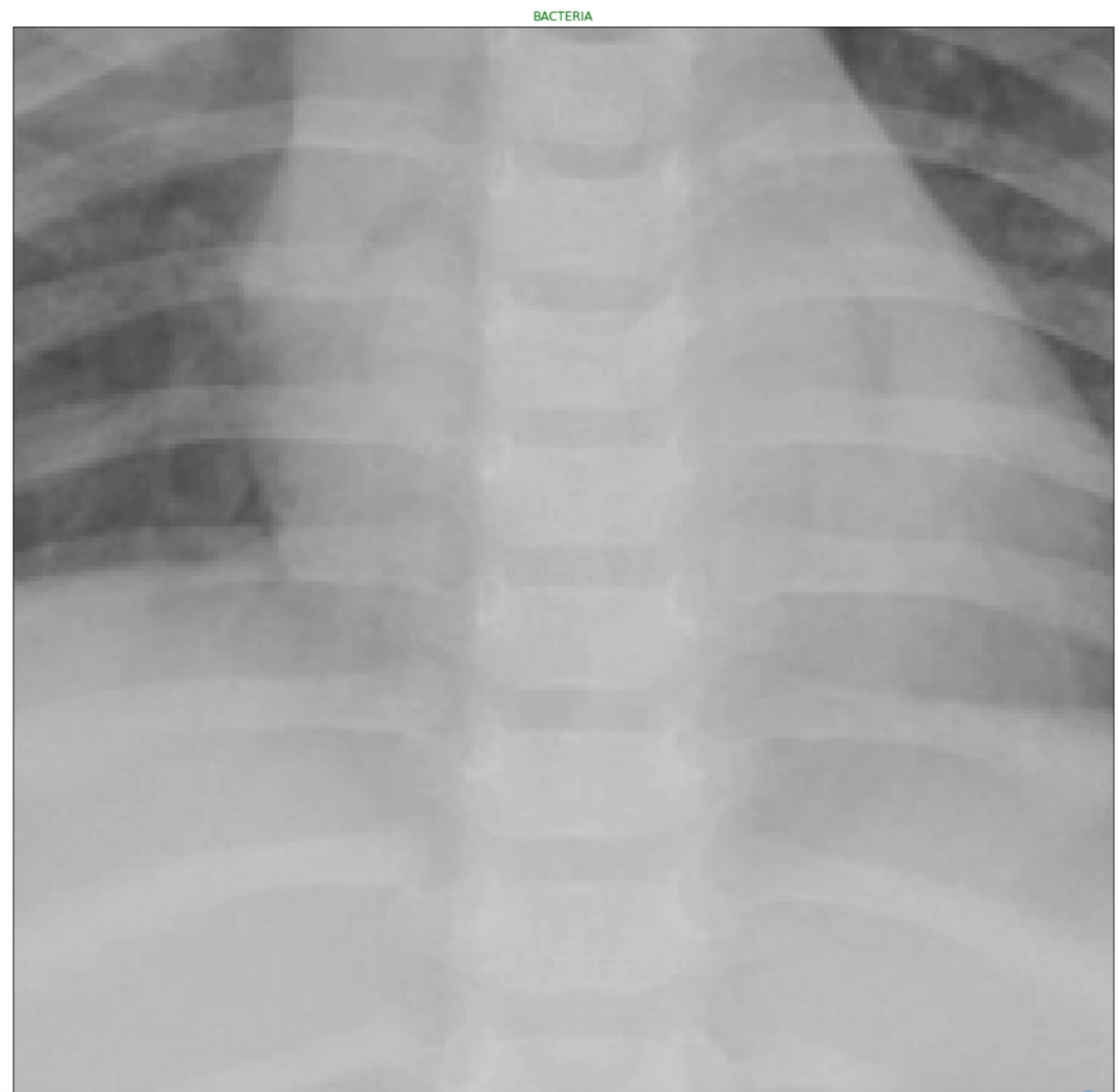
Bacterial pneumonia (BACTERIA)
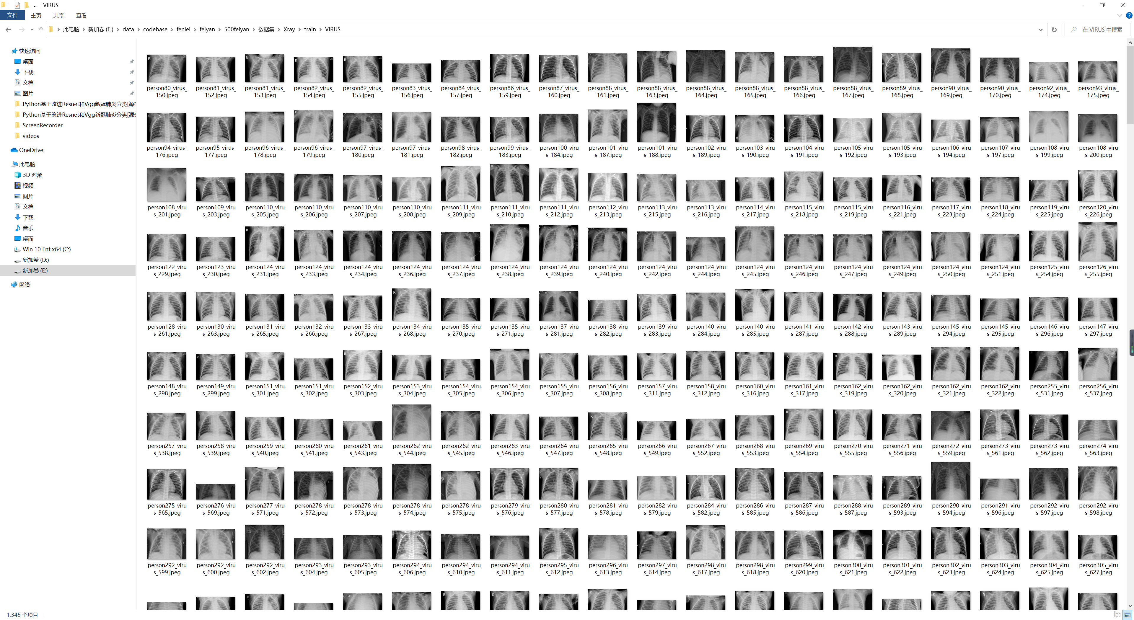
Viral pneumonia (VIRUS)
4. Construction of classification network
(1) vgg model
AlexNetAfter the advent, many scholars AlexNetimproved their accuracy by improving the network structure, mainly in two directions: small convolution kernel and multi-scale. The VGGauthors chose another direction, that is, deepening the depth of the network .
Therefore, the vgg model is a model that deepens the depth of the network AlexNet.
So what is the AlexNet model
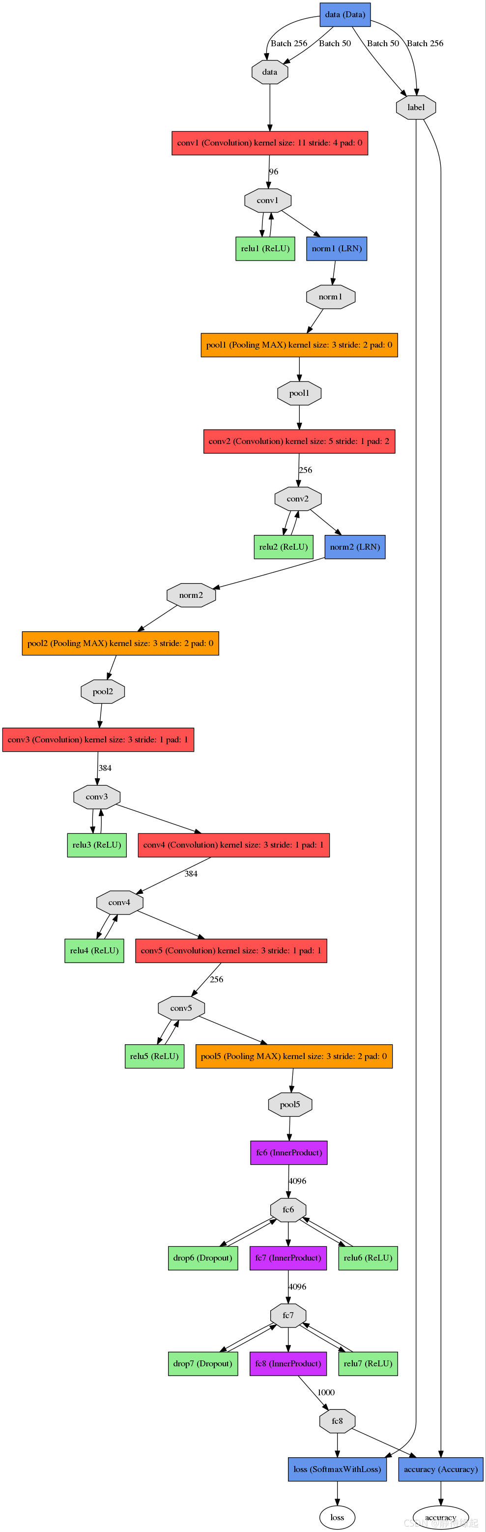
The total number of layers in the network is 8 layers, 5 layers of convolution layers, and 3 layers of fully connected layers .
(2) Resnet model
When the number of neural network layers is relatively high, it is difficult to train, and problems such as gradient explosion and gradient disappearance are prone to occur. Residual network is a kind of skip connection network, which avoids gradient explosion and gradient disappearance and trains deeper network by skipping the previous activation value in the middle network layer and directly passing it to the later network.
When the accuracy of a neural network has reached saturation, increasing the number of network layers may lead to gradient explosion and gradient disappearance, resulting in a sudden drop in accuracy.
Gradient explosion: the activation value will become larger and larger - underfitting
Residual block structural characteristics
During forward calculation: first cache the input matrix of the convolutional layer in the downsample function, and then add
it to the output layer of the convolutional layer. Add resnet to vgg model
step
Put the convolutional structure into the residual block first - pay attention to the number of inputs! = number of outputs, 1*1 convolution dimension transformation, the residual structure is cached in the downsample private function, the forward calculation function outputs out = f (convolution) + identify (dewnsaple)
sequentially writes out the vgg convolution structure, before Torch will automatically call the forward function in the block class after the calculation is written
. Deep understanding of ResNet
First, answer the first question, why does the deep neural network degenerate?
For example: if the optimal network layer number of a neural network is 18 layers, but we do not know how many layers are the optimal solution when designing, based on the idea that the deeper the number of layers, the better, we designed 32 layers, then 14 layers of the 32-layer neural network are actually redundant. If we want to achieve the optimal effect of the 18-layer neural network, we must ensure that the extra 14-layer network must be subjected to identity mapping. The meaning of identity mapping That is to say, what is input, what is output, can be understood as a function such as F(x)=x, because only after such an identity mapping can we ensure that the extra 14 layers of neural network will not affect our optimal Effect.
An explanation for the phenomenon of gradient explosion The
actual optimal number of layers in the network should be before the number of designed layers. After a few more layers, the loss will increase as the parameters continue to optimize (training to exceed the optimal number of layers), but it is
realistic The parameters of the neural network are all trained. It is actually very difficult to ensure that the trained parameters can accurately complete the identity mapping of F(x)=x. It’s good if the number of extra layers is small, and it will not have a great impact on the effect, but if there are too many extra layers, the result may not be very ideal. At this time, the great gods proposed the ResNet residual neural network to solve the problem of neural network degradation.
Why does adding a residual block prevent the neural network degradation problem?
Let's take a look at what the function we said earlier to complete the identity mapping looks like after adding the residual block. Does it become h(X)=F(X)+X, we want to make h(X)=X, then is it equivalent to only need to make F(X)=0, here is clever! It is much easier for a neural network to become 0 through training than to become X, because everyone knows that when we generally initialize the parameters of the neural network, we set a random number between [0, 1]. Therefore, it is easy to approach 0 after network transformation. For example:
Suppose the network is only linearly transformed, with no bias and no activation function. We found that because the random initialization weights are generally biased towards 0, the output value of the network is [0.6 0.6], which is obviously closer to [0 0] than [2 1], compared to learning h(x) =x, the model is faster to learn F(x)=0.
And ReLU can activate negative numbers to 0, filter the linear changes of negative numbers, and make F(x)=0 faster. In this way, when the network decides which network layers are redundant layers, the network using ResNet largely solves the problem of learning the identity mapping, and uses the learning residual F(x)=0 to update the parameters of the redundant layer instead Learning h(x)=x updates the parameters of the redundant layer.
In this way, when the network decides which layers are redundant layers, the network of this layer is identically mapped to the input of the previous layer by learning the residual F(x)=0, so that the network effect with these redundant layers is different from that without. The network effect of these redundant layers is the same, which largely solves the problem of network degradation.
5. Code implementation
class VGG16(nn.Module):
    def __init__(self):
        super(VGG16, self).__init__()
        self.features = nn.Sequential(
            # conv1
            nn.Conv2d(3, 64, 3, 1, 1),
            nn.BatchNorm2d(64, 0.9),
            nn.ReLU(),
            nn.Conv2d(64, 64, 3, 1, 1),
            nn.BatchNorm2d(64, 0.9),
            nn.ReLU(),
            nn.MaxPool2d(2, 2),
            # conv2
            nn.Conv2d(64, 128, 3, 1, 1),
            nn.BatchNorm2d(128, 0.9),
            nn.ReLU(),
            nn.Conv2d(128, 128, 3, 1, 1),
            nn.BatchNorm2d(128, 0.9),
            nn.ReLU(),
            nn.MaxPool2d(2, 2),
            # conv3
            nn.Conv2d(128, 256, 3, 1, 1),
            nn.BatchNorm2d(128, 0.9),
            nn.ReLU(),
            nn.Conv2d(256, 256, 3, 1, 1),
            nn.BatchNorm2d(256, 0.9),
            nn.ReLU(),
            nn.Conv2d(256, 256, 3, 1, 1),
            nn.BatchNorm2d(256, 0.9),
            nn.ReLU(),
            nn.MaxPool2d(2, 2),
            # conv4
            nn.Conv2d(256, 512, 3, 1, 1),
            nn.BatchNorm2d(512, 0.9),
            nn.ReLU(),
            nn.Conv2d(512, 512, 3, 1, 1),
            nn.BatchNorm2d(512, 0.9),
            nn.ReLU(),
            nn.Conv2d(512, 512, 3, 1, 1),
            nn.ReLU(),
            nn.MaxPool2d(2, 2),
            # conv5
            nn.Conv2d(512, 512, 3, 1, 1),
            nn.BatchNorm2d(512, 0.9),
            nn.ReLU(),
            nn.Conv2d(512, 512, 3, 1, 1),
            nn.BatchNorm2d(512, 0.9),
            nn.ReLU(),
            nn.Conv2d(512, 512, 3, 1, 1),
            nn.BatchNorm2d(512, 0.9),
            nn.ReLU(),
            nn.MaxPool2d(2, 2)
            )

        self.classifier = nn.Sequential(
            # fc1
            nn.Linear(512, 4096),
            nn.ReLU(),
            nn.Dropout(),
            # fc2
            nn.Linear(4096, 4096),
            nn.ReLU(),
            nn.Dropout(),
            # fc3
            nn.Linear(4096, 1000),
        )

    def forward(self, x):
        x = self.features(x)
        x = x.view(x.size(x), -1)
        x = self.classifier(x)
        return x

net=VGG16()
print(net)
The first layer: convolution layer 1, the input is 224 × 224 × 3 224 \times 224 \times 3 224 × 224 × 3 images, the number of convolution kernels is 96, and the two GPUs in the paper calculate 48 kernels respectively; The size of the convolution kernel is 11 × 11 × 3 11 \times 11 \times 3 11×11×3; stride = 4, stride indicates the step size, pad = 0, indicates that the edge is not expanded;
the size of the graph after convolution What is it like?
wide = (224 + 2 * padding - kernel_size) / stride + 1 = 54
height = (224 + 2 * padding - kernel_size) / stride + 1 = 54
dimention = 96
then proceed (Local Response Normalized), followed by pooling pool_size = (3, 3), stride = 2, pad = 0 Finally, the feature map of the first layer of convolution is obtained. The
final output of the first layer of convolution is
The second layer: convolution layer 2, the input is the feature map of the previous layer of convolution, the number of convolutions is 256, and the two GPUs in the paper have 128 convolution kernels respectively. The size of the convolution kernel is: 5 × 5 × 48 5 \times 5 \times 48 5×5×48; pad = 2, stride = 1; then do LRN, and finally max_pooling, pool_size = (3, 3), stride = 2;
The third layer: convolution 3, the input is the output of the second layer, the number of convolution kernels is 384, kernel_size = ( 3 × 3 × 256 3 \times 3 \times 256 3×3×256), padding = 1, The third layer does not do LRN and Pool
Fourth layer: convolution 4, the input is the output of the third layer, the number of convolution kernels is 384, kernel_size = ( 3 × 3 3 \times 3 3×3), padding = 1, the same as the third layer, no LRNs and Pools
Fifth layer: convolution 5, the input is the output of the fourth layer, the number of convolution kernels is 256, kernel_size = ( 3 × 3 3 \times 3 3×3), padding = 1. Then go directly to max_pooling, pool_size = (3, 3), stride = 2;
The 6th, 7th, and 8th layers are fully connected layers, the number of neurons in each layer is 4096, and the final output softmax is 1000, because as mentioned above, the number of classifications in the ImageNet competition is 1000. RELU and Dropout are used in the fully connected layer.
class ResBlock(nn.Module):
    def __init__(self, input_channels, out_channels, kernel_size):
        super(ResBlock, self).__init__()

        self.function=nn.Sequential(
            nn.Conv2d(input_channels, out_channels, kernel_size, padding=1),
            nn.Conv2d(out_channels, out_channels, kernel_size, padding=1)
        )

        self.downsample=nn.Sequential(
            nn.Conv2d(input_channels,out_channels,kernel_size,padding=1)
        )

    def forward(self, x):
        identify = x
        identify=self.downsample(identify)

        f = self.function(x)
        out = f + identify
        return out
# 首先将vgg第一层卷积代码加入残差块结构
class My_Model_Blook(nn.Module):
    def __init__(self,input_channels, out_channels, kernel_size):  # 3 64 3
        super(My_Model_Blook, self).__init__()
        self.function = nn.Sequential(
            nn.Conv2d(input_channels, out_channels, kernel_size, 1, 1),
            nn.BatchNorm2d(out_channels, 0.9),
            nn.ReLU(),
            nn.Conv2d(out_channels, out_channels, kernel_size, 1, 1),
            nn.BatchNorm2d(out_channels, 0.9),
            nn.ReLU(),
            nn.MaxPool2d(2, 2)
        )

        self.downsample = nn.Sequential(
            nn.Conv2d(input_channels, out_channels, kernel_size, 1, 1),
            nn.BatchNorm2d(out_channels, 0.9),
            nn.ReLU(),
            nn.MaxPool2d(2, 2),
            # nn.Conv2d(out_channels, out_channels, kernel_size, 1, 1),
            # nn.BatchNorm2d(out_channels, 0.9),
            # nn.ReLU(),
            # nn.MaxPool2d(2, 2)
        )


    def forward(self, x):
        identify = x
        identify = self.downsample(identify)
        f = self.function(x)

        # print(f"f:{f.size()}  identify:{identify.size()}")

        out = f + identify
        return out

# 将残差块代码封装复用
class My_Model(nn.Module):
    def __init__(self,in_channels=3, num_classes=10):
        super(My_Model, self).__init__()
        self.conv1 = nn.Sequential(
            My_Model_Blook(3,64,3)
        )
        self.conv2 = nn.Sequential(
            My_Model_Blook(64, 128, 3)
        )
        self.conv3 = nn.Sequential(
            My_Model_Blook(128, 256, 3)
        )
        self.conv4 = nn.Sequential(
            My_Model_Blook(256, 512, 3)
        )

        # bug:输入输出一致时不能用1*1卷积,会发生维度消失,无法衔接后面模型
        # 解决方法:在残差块中不加1*1卷积或者单独卷积

        # self.conv5 = nn.Sequential(
        #     My_Model_Blook(512, 512, 3)
        # )


        self.classifier = nn.Sequential(
            # fc1
            nn.Linear(512, 1024),
            nn.ReLU(),
            nn.Dropout(),
            # fc2
            nn.Linear(1024, 1024),
            nn.ReLU(),
            nn.Dropout(),
            # fc3
            nn.Linear(1024, num_classes),
        )
    def forward(self, x):
        out = self.conv1(x)
        out = self.conv2(out)
        out = self.conv3(out)
        out = self.conv4(out)

        # bug:输入输出一致时不能用1*1卷积,会发生维度消失,无法衔接后面模型

        # print(out.size())
        # out = self.conv5(out)
        # print(out.size())
        # out = out.resize(512,1,1)

        out = out.view((x.shape[0], -1))  # 拉成一维
        out = self.classifier(out)
        return out
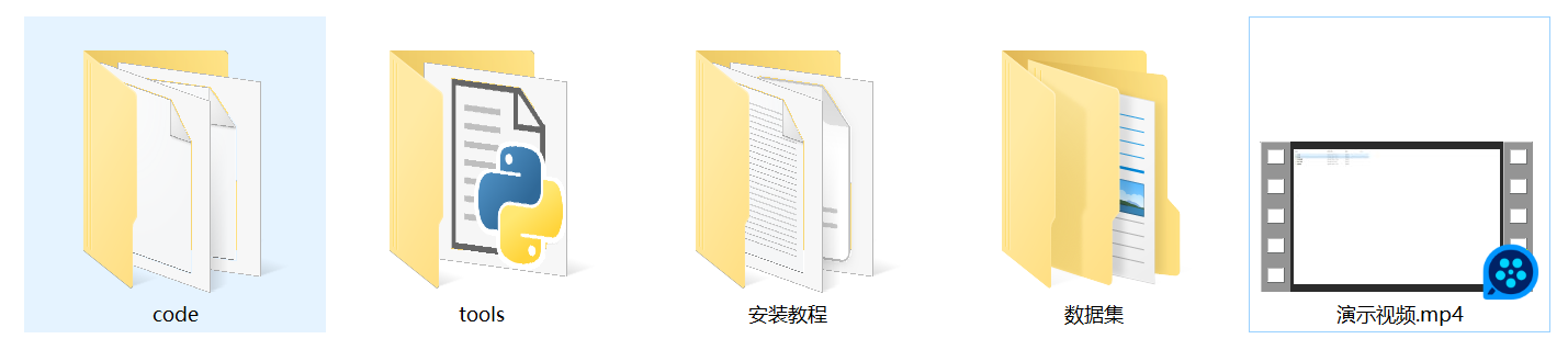
6. Complete project display
7. Complete project download
Baidu Bread can download the source code by searching for the title name
8. References
[1] S. Madhogaria et al., Pixel-based classifification method for detecting unhealthy regions in leaf images, GI-Jahrestagung. (2011).
[2] A.l. Bashish, M.B. Dheeb, S. Bani-Ahmad, A framework for detection and
classifification of plant leaf and stem diseases, 2010 International Conference on Signal and Imageprocessing, IEEE, 2010.
[3] P. Revathi, M. Hemalatha, Advance computing enrichment evaluation of cotton leaf spot disease detection using image edge detection, 2012 Third
International Conference on Computing, Communication and Networking
Technologies (ICCCNT’12), IEEE, 2012.
[4] P.S. Landge et al., Automatic detection and classifification of plant disease through image processing, Int. J. Adv. Res. Comp. Sci. Softw. Eng. 3 (7) (2013) 798–801.
[5] M. Ranjan et al., Detection and classifification of leaf disease using artifificial neural network, Int. J. Techn. Res. Appl. 3 (3) (2015) 331–333.
[6] B.S. Prajapati, V.K. Dabhi, H.B. Prajapati, A survey on detection and
classifification of cotton leaf diseases, 2016 International Conference on
Electrical, Electronics, and Optimization Techniques (ICEEOT), IEEE, 2016.
[7] A. Khamparia, G. Saini, D. Gupta, A. Khanna, S. Tiwari, V.H.C. de Albuquerque, Seasonal crops disease prediction and classifification using deep convolutional encoder network, Circ. Syst. Sign. Process. 39 (2) (2020) 818–836.
[8] S.P. Mohanty, D.P. Hughes, M. Salathé, Using deep learning for image-based plant disease detection, Front. Plant Sci. 7 (2016) 1419.
[9] P. Gong, C. Zhang, M. Chen, Deep learning for toxicity and disease prediction, Front. Genet. 11 (2020) 175.