2022 Shenzhen Cup C Autonomous Driving Electric Material Vehicle Swap Station Site Selection and Scheduling Scheme
In order to achieve my country's goal of "carbon peaking" by 2030 and "carbon neutrality" by 2060, the use of environmentally friendly self-driving electric vehicles in material transportation is a development trend. When formulating the electric vehicle dispatching plan, the time cost of charging and replacing the battery must be considered, and a new vehicle transportation location selection and dispatching problem is proposed.
Question 1 A batch of self-driving electric material trucks transports materials from point P to point D, and then returns empty-loaded, and
so on and so forth. It is required to establish a mathematical programming model to determine the location of a two-way co-located (like a high-speed rest station) swap station between point P and point D, as well as the corresponding vehicle and battery pack scheduling scheme to maximize the delivery within the specified time period. The amount of material meets resource constraints and battery operating mode constraints. According to the data given in the appendix, solve the planning model, give the location of the swap station, and give the amount of materials transported in 1000 hours, the number of vehicles used, the number of battery packs, and the specific scheduling scheme of the vehicles and their battery packs.
Question 2 In question 1, change the station construction condition to "determine a position of a power exchange station in each direction between point P and point D", other conditions and tasks are the same as question 1.
Question 3 Considering the costs of peak and valley electricity prices, purchase of battery packs, construction of charging and swapping stations, etc., formulate a station construction and battery pack scheduling plan that guarantees the minimum daily transportation volume and the lowest investment and operation cost in the 3-year settlement cycle. According to the data given in the appendix (the default data is supplemented by itself), a specific calculation example is given. Problem 4 For multiple pick-up points and a single unloading point, study the above-mentioned swap station site selection and vehicle-battery group scheduling problems.
Appendix: Data Format (Limited)
The calculation example data is compiled by itself under the following format restrictions, and the unified test calculation example data will be released before the finals.
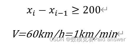
(1) Point P to Point D: mileage 10 km, two-way single-vehicle (rail) dedicated lane, vehicle distance not less than 200 m
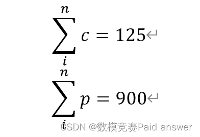
(2) Vehicles: 125 vehicles at a speed of 60 km/h, each vehicle is rated with 6 battery packs, Initially in the no-load state of the swap station, and the SoC (state of charge) of each on-board battery pack is 100%
(3) Batteries: 900 groups, a single battery group is independently metered, the power consumption of the 6 battery groups in the vehicle is consistent, the SoC of each battery group is reduced by 1% every 3 minutes of driving an empty vehicle, and the SoC of each battery group is reduced by 1% every 2 minutes that a truck The SoC of the battery pack is reduced by 1%. The SoC of the on-board battery pack can be replaced when it is in the interval [10%, 25%]. The SoC of the battery pack for replacement is 100%
. It takes 20 seconds for each battery pack to be charged and detected to enter the standby state after being replaced. It takes 1 minute each time for loading and unloading
. Automatic battery replacement equipment price, battery price, vehicle price.
Model establishment and solution analysis:
The first thing to consider is this question: from the power exchange station to point P to point D to point P until the battery capacity reaches 10% to 25%, go to the power exchange station for battery replacement
. Here you can draw a circuit diagram
The length of the S double-lane road is 10km, that is, 10,000m
, and the distance between two vehicles is greater than or equal to 200m. What does it mean?
There are at most 100 Benz trams on the road without considering the length of the car. The
question said that the battery: 900 groups, a single battery group is independently measured, and the 6 on-board battery groups consume the same amount of power.
I don’t have enough IQ balance. I don’t consider the situation of charging 6 batteries in batches and replacing batteries in batches. I directly write in the assumptions of the model: Suppose the electric car is replaced by the battery and the 6 battery packs are replaced together, ignoring that a single battery is replaced individually. The impact of cargo capacity.
It is also the battery replacement in batches, and the location of the replacement station, the maximum freight volume, and the time 1000h=60000min, the difference between 6 batteries used close to 10% and replaced in batches. I know that it will affect the overall 900 groups. The usage rate of the battery, but this battery replacement program is not easy to calculate. The meaning of this question is to ask you to use a combination of integer programming and linear programming. There are 100 trams running on the road, and the rest of the batteries are charged without wasting as much as possible. Then the battery is just fully charged when the car runs to 10%. This cycle goes back and forth, ask you where to build the power station? How to change the battery? The maximum cargo volume can be achieved.
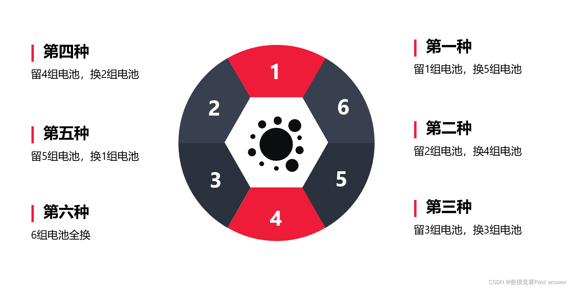
Let me tell you why the location of the power station is easy to calculate but the battery replacement distribution scheme is not. This is because if you have 6 batteries, if you have a battery replacement scheme, you have C6 to choose 1, that is, 6 battery replacement schemes, and then you compare or It is the IQ that rolls out the optimal battery replacement solution. Why are there 6 solutions? Because 25%-10%=15% of the electricity can run back and forth to add another electricity or return electricity, but you have to ensure that you have the remaining electricity to go to the power station, so you can't go the second time, you can only change it honestly electricity, understand?
Final result
The first question and finally you confirm that the swap station is to build a swap station 5km from P to D. As for the battery replacement plan, guess how you can use the entire battery to maximize the efficiency? The transportation volume is related to the number of cars and the number of times the tram reaches P, and the battery affects the number of cars and the number of times to P. Dear reader, have you turned this corner?
The final result of the second question is to build a power exchange station at 20/3km from the going and returning.
The third question results need to consider the time point of the change point, how to change the day and night, how to use the industrial electricity time, the lowest price and the highest price of the power exchange strategy plan
The fourth question results need to consider the queuing theory algorithm
idea is finally completed
The above only represents my personal understanding of the subject
Program code example:
import math # 导⼊模块
import random # 导⼊模块
import pandas as pd # 导⼊模块 YouCans, XUPT
import numpy as np # 导⼊模块 numpy,并简写成 np
import matplotlib.pyplot as plt
from datetime import datetime
# ⼦程序:定义优化问题的⽬标函数
def cal_Energy(X, nVar, mk): # m(k):惩罚因⼦,随迭代次数 k 逐渐增⼤
p1 = (max(0, 6*X[0]+5*X[1]-60))**2
p2 = (max(0, 10*X[0]+20*X[1]-150))**2
fx = -(10*X[0]+9*X[1])
return fx+mk*(p1+p2)
# ⼦程序:模拟退⽕算法的参数设置
def ParameterSetting():
cName = "funcOpt" # 定义问题名称 YouCans, XUPT
nVar = 2 # 给定⾃变量数量,y=f(x1,..xn)
xMin = [0, 0] # 给定搜索空间的下限,x1_min,..xn_min
xMax = [8, 8] # 给定搜索空间的上限,x1_max,..xn_max
tInitial = 100.0
tFinal = 1
alfa = 0.98
meanMarkov = 100 # Markov链长度,也即内循环运⾏次数
scale = 0.5 # 定义搜索步长,可以设为固定值或逐渐缩⼩
return cName, nVar, xMin, xMax, tInitial, tFinal, alfa, meanMarkov, scale
# 模拟退⽕算法
def OptimizationSSA(nVar,xMin,xMax,tInitial,tFinal,alfa,meanMarkov,scale):
# ====== 初始化随机数发⽣器 ======
randseed = random.randint(1, 100)
random.seed(randseed) # 随机数发⽣器设置种⼦,也可以设为指定整数
# ====== 随机产⽣优化问题的初始解 ======
xInitial = np.zeros((nVar)) # 初始化,创建数组
for v in range(nVar):
# xInitial[v] = random.uniform(xMin[v], xMax[v]) # 产⽣ [xMin, xMax] 范围的随机实数
xInitial[v] = random.randint(xMin[v], xMax[v]) # 产⽣ [xMin, xMax] 范围的随机整数
# 调⽤⼦函数 cal_Energy 计算当前解的⽬标函数值
fxInitial = cal_Energy(xInitial, nVar, 1) # m(k):惩罚因⼦,初值为 1
# ====== 模拟退⽕算法初始化 ======
xNew = np.zeros((nVar)) # 初始化,创建数组
xNow = np.zeros((nVar)) # 初始化,创建数组
xBest = np.zeros((nVar)) # 初始化,创建数组
xNow[:] = xInitial[:] # 初始化当前解,将初始解置为当前解
xBest[:] = xInitial[:] # 初始化最优解,将当前解置为最优解
fxNow = fxInitial # 将初始解的⽬标函数置为当前值
fxBest = fxInitial # 将当前解的⽬标函数置为最优值
print('x_Initial:{:.6f},{:.6f},\tf(x_Initial):{:.6f}'.format(xInitial[0], xInitial[1], fxInitial))
recordIter = [] # 初始化,外循环次数
recordFxNow = [] # 初始化,当前解的⽬标函数值
recordFxBest = [] # 初始化,最佳解的⽬标函数值
recordPBad = [] # 初始化,劣质解的接受概率
kIter = 0 # 外循环迭代次数
totalMar = 0 # 总计 Markov 链长度
totalImprove = 0 # fxBest 改善次数
nMarkov = meanMarkov # 固定长度 Markov链
# ====== 开始模拟退⽕优化 ======
# 外循环
tNow = tInitial # 初始化当前温度(current temperature)
while tNow >= tFinal: # 外循环

kBetter = 0 # 获得优质解的次数
kBadAccept = 0 # 接受劣质解的次数
kBadRefuse = 0 # 拒绝劣质解的次数
# ---内循环,循环次数为Markov链长度
for k in range(nMarkov): # 内循环,循环次数为Markov链长度
totalMar += 1 # 总 Markov链长度计数器
# ---产⽣新解
# 产⽣新解:通过在当前解附近随机扰动⽽产⽣新解,新解必须在 [min,max] 范围内
# ⽅案 1:只对 n元变量中的⼀个进⾏扰动,其它 n-1个变量保持不变
xNew[:] = xNow[:]
v = random.randint(0, nVar-1) # 产⽣ [0,nVar-1]之间的随机数
xNew[v] = round(xNow[v] + scale * (xMax[v]-xMin[v]) * random.normalvariate(0, 1))
# 满⾜决策变量为整数,采⽤最简单的⽅案:产⽣的新解按照四舍五⼊取整
xNew[v] = max(min(xNew[v], xMax[v]), xMin[v]) # 保证新解在 [min,max] 范围内
# ---计算⽬标函数和能量差
# 调⽤⼦函数 cal_Energy 计算新解的⽬标函数值
fxNew = cal_Energy(xNew, nVar, kIter)
deltaE = fxNew - fxNow
# ---按 Metropolis 准则接受新解
# 接受判别:按照 Metropolis 准则决定是否接受新解
if fxNew < fxNow: # 更优解:如果新解的⽬标函数好于当前解,则接受新解
accept = True
kBetter += 1
else: # 容忍解:如果新解的⽬标函数⽐当前解差,则以⼀定概率接受新解
pAccept = math.exp(-deltaE / tNow) # 计算容忍解的状态迁移概率
if pAccept > random.random():
accept = True # 接受劣质解
kBadAccept += 1
else:
accept = False # 拒绝劣质解
kBadRefuse += 1
# 保存新解
if accept == True: # 如果接受新解,则将新解保存为当前解
xNow[:] = xNew[:]
fxNow = fxNew
if fxNew < fxBest: # 如果新解的⽬标函数好于最优解,则将新解保存为最优解
fxBest = fxNew
xBest[:] = xNew[:]
totalImprove += 1
scale = scale*0.99 # 可变搜索步长,逐步减⼩搜索范围,提⾼搜索精度
# ---内循环结束后的数据整理
#
pBadAccept = kBadAccept / (kBadAccept + kBadRefuse) # 劣质解的接受概率
recordIter.append(kIter) # 当前外循环次数
recordFxNow.append(round(fxNow, 4)) # 当前解的⽬标函数值
recordFxBest.append(round(fxBest, 4)) # 最佳解的⽬标函数值
recordPBad.append(round(pBadAccept, 4)) # 最佳解的⽬标函数值
The idea is finally completed, welcome to disturb