Articles copied from know almost - Wanggui Bo
This paper describes the convolution Convolution background, the basic principles, characteristics, and the difference between the full link connection, different convolution mode, and a convolutional code to achieve the visualization of a simple two-dimensional convolution operation, and for the volume It was calculated to optimize product operation.
table of Contents
- Convolution background and principle
- It features convolution (the difference between full-contact connection)
- Three modes of convolution
- Convolution operation
Numpysimple implementation - Optimized for convolution
Convolution background and principle
Convolution operation history up to the development of signal processing in the signal processing will usually be mixed with the original signal noise, sensor assumed at each instant \ (T \) outputs a signal \ (F (T) \) , this signal is usually mixed with some of the noise, we can cancel out noise weighted average over by measurement points, and the current time from the point \ (T \) closer measurement points higher weights would, we can be represented by the following formula
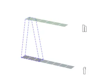
The formula \ (G \) is a weighting function, the parameter is the time point \ (t '\) from the current time \ (T \) from the output (\ \ t') the right point in time measured weight; \ (F \) is the signal measurement functions. In this example, \ (T '\) sampling is discrete, so using plus and forms, while \ (G \) should also be a probability density function, as expressed a weight in this case. The figure is an example of the visualization, in gray \ (F (T) \) , the red part is inverted through \ (G \) , the green part is generated \ (H \) .
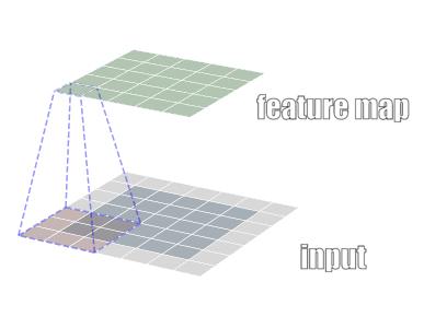
This example is actually a special case of the convolution operation is further extended to a continuous function, and to \ (G \) function is not limited, and we get the definition of the convolution operation. According to Wikipedia defined convolution ( Convolution) is a two functions G \ (F \) and \ (G \) generating a third function \ (F \) is a mathematical operator, the formula is expressed as follows. The function is generally referred to as input
input( ), a function called convolution kernel
kernel( ) function is called characteristic map
feature map( )
We consider the case of a multi-dimensional discrete convolution, the most common of the depth of field of study is the case, the input is a multi-dimensional array, convolution kernel is a multi-dimensional array, the time is discrete and infinite points become limited array finite element and add:
Formula indicated intuitively understanding the operation of the convolution kernel to be inverted, and then multiply the input point summation output. In the field of machine learning, especially learning in depth, to achieve convolution convolution kernel is usually omitted flip this step, since the convolution kernel parameters depth of learning is learning updated, so there is no reversal does not affect the properties. Strictly defined, the depth of learning is actually another convolution operation: cross-correlation Cross-Correlation . Formulated as follows
In the following we ignore whether convolution kernel is flipped, the cross-correlation and convolution in the strict sense are called convolution. The two-dimensional convolution visualized as FIG.
It features convolution (the difference between full-contact connection)
Convolution neural network ( Convotional Neural Network, CNN) is the depth of field of study is important in a field, it can be said the success of CNN made in recent years in the field of computer vision directly contributed to the revival of the depth of learning. CNN is a convolution neural network based, can be roughly understood as CNN is connected to the whole network into convolution matrix multiplication (generally because coarse said CNN further pooling with other proprietary CNN operating). So what are the characteristics different from the convolution operation fully connected it?
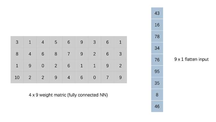
We look at an example of specific convolution
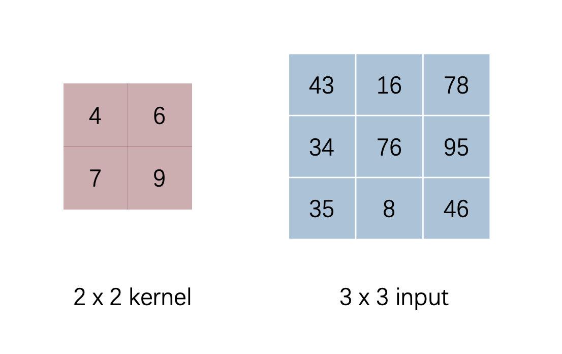
Irrespective of padding, with a stride of 1, we calculated the result of the convolution of
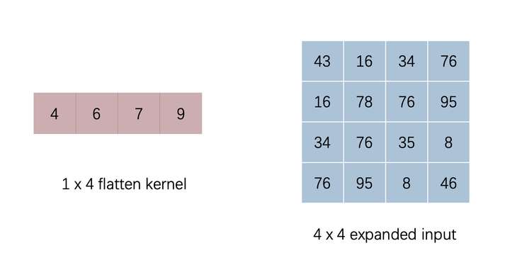
We are converting input and kernel in the figure, input flattened into a vector, kernel where appropriate zero fill
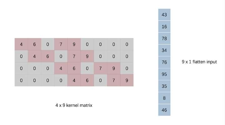
After this treatment actually left on the right side of the kernel matrix multiplied by the vector flatten input result obtained is equivalent to the above results, i.e. the vector convolution operation may be represented by a vector on a core matrix of FIG obtained. There did not feel very familiar? Such a matrix multiplication parameters obtained in the form of an input vector and the output vector a full connection is completely consistent .
Convolution and therefore full connectivity are essentially a set of linear transformations , but compared in terms of the whole connection convolution, which is more sparse matrix parameters, kernel matrix many zero (sparse connectivity), while the parameters actually nonzero It is shared (parameter sharing). These two features allow convolution can greatly reduce the number of parameters, while the same set of parameters (convolution kernel) reuse in multiple places more conducive to capture local characteristics . In contrast parameters more fully connected, each parameter is only responsible for a unique connection, computational, memory requirements increase but also more difficult to train.
More Essentially, compared to full convolution is actually connected parameter matrix made a priori limitation (the matrix is sparse, while the parameter multiplexing), which is based on the prior phase in a high-dimensional space basis of a certain relationship of adjacent data points, such as between a partial image may constitute a shape or a component, so that the convolution operation is particularly suitable for the image data. While the addition of such a priori loss model will fit a certain ability, but the final results from the point of view of the benefits are far greater than the loss of the ability to fit.
Three modes of convolution
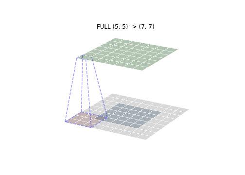
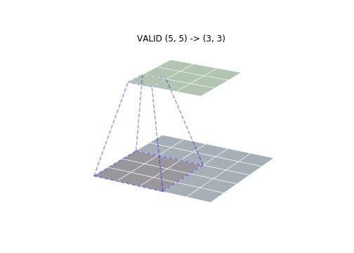
Depth learning framework typically implement convolutional three different modes, namely SAME, VALID, FULL. Core difference among these three modes is different convolving a convolution operation of the mobile core region , leading to different output sizes. We distinguish three modes of an example of view, the size of the input picture is , convolution kernel size
, stride to take 1.
- FULL mode
FULL mode convolution kernel from the input there is a point of intersection where to start convolution . , The position of the blue box is a convolution kernel convolution first place, the gray portion is below the normal to the convolution performed padding (fill typically 0). Therefore, the maximum size of the convolution kernel convolution output moving area FULL mode is also the largest.
- VALID mode
FULL VALID mode and a mode contrary, where the convolution kernel with the input entire overlap began convolution , the size does not require padding, the output is minimal
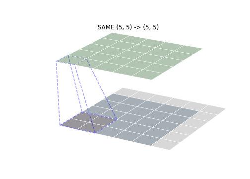
- SAME mode
SAME mode is the most common mode, SAME mean size convolution output with the input size is consistent (assuming a stride of 1). Aligned convolution start position determined by the first input center point of the convolution kernel, then filled to the corresponding padding. As shown below, it can be seen that the size of the convolution output was consistent access.
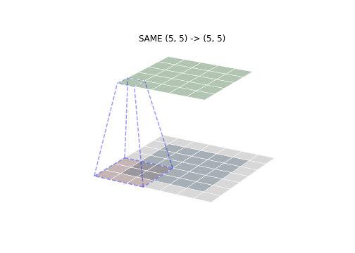
When the convolution kernel mode SAME side length is an even number, where one side can increase the number of row (column) padding, padding i.e. asymmetrical output achieve consistent size and dimensions of input, as shown below (FIG convolution kernel size )
These three different modes except that the convolution operation of convolving the moving area, in fact, to determine the required padding. Padding each mode is calculated as follows
def get_padding(inputs, ks, mode="SAME"):
    """
    Return padding list in different modes.
    params: inputs (input array)
    params: ks (kernel size) [p, q]
    return: padding list [n,m,j,k]
    """
    pad = None
    if mode == "FULL":
        pad = [ks[0] - 1, ks[1] - 1, ks[0] - 1, ks[1] - 1]
    elif mode == "VALID":
        pad = [0, 0, 0, 0]
    elif mode == "SAME":
        pad = [(ks[0] - 1) // 2, (ks[1] - 1) // 2,
               (ks[0] - 1) // 2, (ks[1] - 1) // 2]
        if ks[0] % 2 == 0:
            pad[2] += 1
        if ks[1] % 2 == 0:
            pad[3] += 1
    else:
        print("Invalid mode")
    return pad
Size determines the size of the input, the convolution kernel size, padding and a stride of, the output was determined, it can be calculated by the following equation. Which are the output, input dimensions,
is the convolution kernel size,
respectively, both sides of the padding.
Convolution operation Numpy simple implementation
After deconvolution operation principle, in fact, very simple to implement, we can use the code to achieve the two-dimensional convolution operation, as follows
def conv(inputs, kernel, stride, mode="SAME"):
    ks = kernel.shape[:2]
    # get_padding
    pad = get_padding(inputs, ks, mode="SAME")
    padded_inputs = np.pad(inputs, pad_width=((pad[0], pad[2]), (pad[1], pad[3]), (0, 0)), mode="constant")

    height, width, channels = inputs.shape
    out_width = int((width + pad[0] + pad[2] - ks[0]) / stride + 1)
    out_height = int((height + pad[1] + pad[3] - ks[1]) / stride + 1)

    outputs = np.empty(shape=(out_height, out_width))
    for r, y in enumerate(range(0, padded_inputs.shape[0]-ks[1]+1, stride)):
        for c, x in enumerate(range(0, padded_inputs.shape[1]-ks[0]+1, stride)):
            outputs[r][c] = np.sum(padded_inputs[y:y+ks[1], x:x+ks[0], :] * kernel)
    return outputs
Use an image test
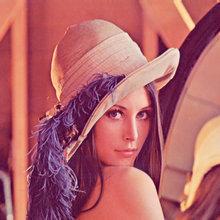
inputs = from_image("./Lenna_test_image.png")
to_image(inputs, save_path="./plots/conv/lenna_origin.png")
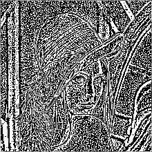
# Embossing Filter
kernel_one_channel = np.array([[0.1, 0.1, 0.1], [0.1, -0.8, 0.1], [0.1, 0.1, 0.1]])
kernel = np.stack([kernel_one_channel] * 3, axis=2)
stride = 1
output = conv(inputs, kernel, stride)
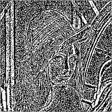
to_image(output, grey=True, save_path="./plots/conv/lenna_conv.png")
After the input image and the convolution following effects.
Convolution operation Numpy simple implementation
We are strictly in accordance with the above procedure convolution implemented (dot -> summation -> Mobile convolution kernel) when discussing the difference between convolution and fully connected in the above mentioned long as we do on the convolution kernel and some input changes, can be equivalently converted to the convolution matrix and vector multiplication, which can improve the efficiency of the convolution calculation. There are two methods converting a convolution kernel extension is filled, the input flattening, the other is a convolution kernel for flattening, filling of the input extension. The final results of the two methods is up, we chose the second option for implementation. The figure is flattened through the convolution of the input vector has been expanded matrix.
ptyhon code to achieve the following
def conv_matmul(inputs, kernel, stride, mode="SAME"):
    ks = kernel.shape[:2]

    pad = get_padding(inputs, ks, mode=mode)
    padded_inputs = np.pad(inputs, pad_width=((pad[0], pad[2]), (pad[1], pad[3]), (0, 0)), mode="constant")

    height, width, channels = inputs.shape
    out_width = int((width + pad[0] + pad[2] - ks[0]) / stride + 1)
    out_height = int((height + pad[1] + pad[3] - ks[1]) / stride + 1)

    rearrange = []
    for y in range(0, padded_inputs.shape[0]-ks[1]+1, stride):
        for x in range(0, padded_inputs.shape[1]-ks[0]+1, stride):
            patch = padded_inputs[y:y+ks[1], x:x+ks[0], :]
            rearrange.append(patch.ravel())
    rearrange = np.asarray(rearrange).T
    kernel = kernel.reshape(1, -1)
    return np.matmul(kernel, rearrange).reshape(out_height, out_width)
To verify the effect of
inputs = from_image("./Lenna_test_image.png")
to_image(inputs, save_path="./plots/conv/lenna_origin.png")

#  Embossing Filter
kernel_one_channel = np.array([[0.1, 0.1, 0.1], [0.1, -0.8, 0.1], [0.1, 0.1, 0.1]])
kernel = np.stack([kernel_one_channel] * 3, axis=2)
stride = 1
output = conv_matmul(inputs, kernel, stride)
to_image(output, grey=True, save_path="./plots/conv/lenna_conv.png")
Run time in comparison with the original implementation of optimized
n = 5

start = time.time()
for _ in range(n):
    output = conv(inputs, kernel, stride=1)
cost1 = float((time.time() - start) / n)
print("raw time cost: %.4fs" % cost1)

start = time.time()
for _ in range(n):
    output = conv_matmul(inputs, kernel, stride=1)
cost2 = float((time.time() - start) / n)
print("optimized time cost: %.4fs" % cost2)

reduce = 100 * (cost1 - cost2) / cost1
print("reduce %.2f%% time cost" % reduce)
raw time cost: 0.7281s
optimized time cost: 0.1511s
reduce 79.25% time cost
A first implementation of the test image on the average time 0.7281s, the optimized implementation of the average time 0.1511s, by optimizing the matrix operation can bring about 80% to enhance the operation speed .
Finally, see the relevant code here