Detailed visualization of graph convolution and message passing theory

Reprinted from: Deephub Imba

In this article, we will study how to build a graph convolutional neural network based on a message passing mechanism and create a model to classify molecules with embedded visualizations.

Suppose there is now a need to design drugs to treat certain diseases. There is a dataset of drugs that successfully treat a disease and drugs that don't work, and now we need to design a new drug and want to know if it can treat the disease. If a meaningful representation of a drug can be created, a classifier can be trained to predict whether it will be useful for disease treatment. Our drugs are molecular formulas, which can be represented graphically. The nodes of this graph are atoms. Atoms can also be described by eigenvectors x (which can consist of atomic properties such as mass, number of electrons, or others). To classify molecules, we want to use knowledge about their spatial structure and atomic characteristics to obtain some meaningful representations.

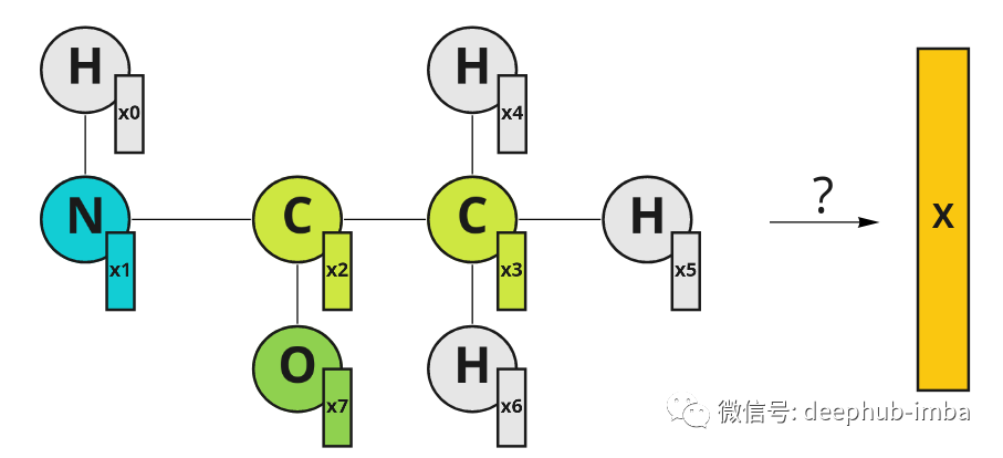
An example of a molecule represented graphically. Atoms have their eigenvectors X. The indices in the feature vector represent the node indices.

The most straightforward way is to aggregate the feature vectors, e.g. simply take their average:

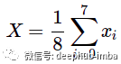
This is a valid solution, but it ignores important molecular spatial structures.

graph convolution

We can come up with another idea: represent the molecular graph with an adjacency matrix and "extend" its depth with eigenvectors. We get a fake image [8, 8, N], where N is the dimension of the node feature vector x. It is now possible to use regular convolutional neural networks and extract molecular embeddings.

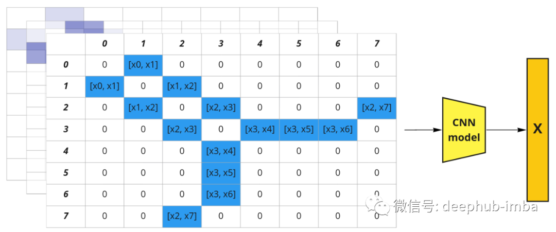
The graph structure can be represented as an adjacency matrix. Node features can be represented as channels in the image (brackets represent connections).

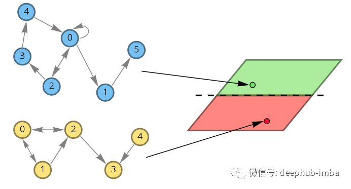
This approach takes advantage of the graph structure, but has a huge disadvantage: if you change the order of the nodes you will get a different representation. So such a representation is not a permutation invariant. But the order of nodes in the adjacency matrix is arbitrary, for example, you can change the column order from [0, 1, 2, 3, 4, 5, 6, 7] to [0, 2, 1, 3, 5, 4, 7, 6], which is still a valid adjacency matrix for the graph. So creating all possible permutations and stacking them together would give us 1625702400 possible adjacency matrices (8!*8!). The amount of data is too large, so a better solution should be found.

But the question is, how do we integrate spatial information and do it efficiently? The above example can make us think of the concept of convolution, but it should be done on a graph.

So graph convolution appears

What happens when a regular convolution is applied to an image? The values of adjacent pixels are multiplied by the filter weights and added. Can we do something similar on the graph? Yes, it is possible to stack node feature vectors in matrix X and multiply them by adjacency matrix A, and then get updated feature X` which incorporates information about node's nearest neighbors. For simplicity, let's consider an example with scalar node features:

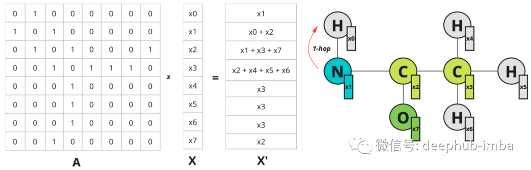
Example of a scalar-valued node feature. The 1-hop distance is specified for node 0 only, but the same is true for all other nodes.

Each node gets information about its nearest neighbor (also known as 1-hop distance). Multiplication on the adjacency matrix propagates features from one node to another.

The receptive field can be expanded in the image domain by increasing the filter size. In the graph, further neighbors can be considered. If you multiply A^2 by X - information about nodes 2 hops away is propagated to nodes:

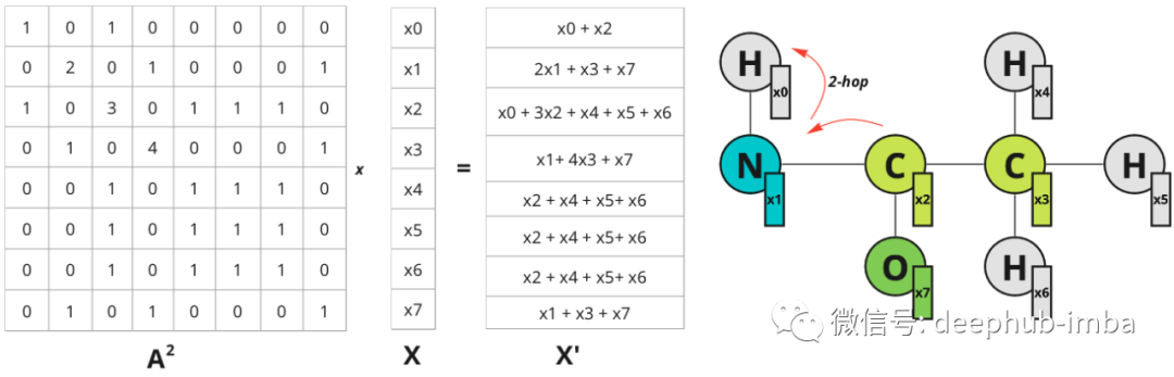
Node 0 now has information about node 2, which is within 2 hops away. The diagram illustrates hops only for node 0, but also for all other nodes.

Higher powers of matrix A behave the same way: multiplying by A^n causes features to propagate from nodes n hops away, so the "receptive field" can be extended by adding multiplication to higher powers of the adjacency matrix. To generalize this operation, the function for node updates can be defined as the sum of such multiplications with some weight w:

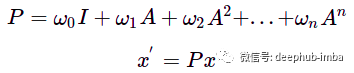
Polynomial graph convolution filter. A - graph adjacency matrix, w - scalar weight, x - initial node feature, x' - updated node feature.

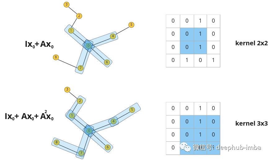
The new feature x' is some mix of nodes from n hops away, the influence of the corresponding distance is controlled by the weight w. Such an operation can be thought of as a graph convolution with a filter P parameterized by a weight w. Similar to convolution on images, graph convolution filters can also have different receptive fields and aggregate information about node neighbors, but the structure of neighbors is not as regular as convolution kernels in images.

Such polynomials are permutation-equivariant like general convolutions. The graph Laplacian can be used instead of an adjacency matrix to transfer eigendifferences rather than eigenvalues between nodes (normalized adjacency matrices can also be used).

The ability to represent graph convolutions as polynomials can be derived from general spectral graph convolutions. For example, filters utilizing Chebyshev polynomials with a graph Laplacian provide an approximation to direct spectral graph convolution [1].

And it can be easily generalized to any dimension of nodal features with the same equation. But in the case of higher dimensions, the node feature matrix X is processed instead of the node feature vector. For example, for N nodes and 1 or M features in a node, we get:

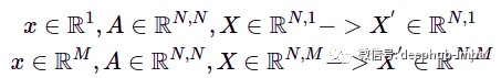
x—node feature vector, X—stacked node feature, M—dimension of node feature vector, N—node number.

The "depth" dimension of a feature vector can be thought of as "channels" in image convolution.

messaging

Now look at the above discussion in a different way. Continuing with a simple polynomial convolution discussed above, with only two first terms, let w equal 1:

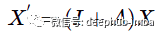
Now if you multiply the graph feature matrix X by (I + A) you get the following result:

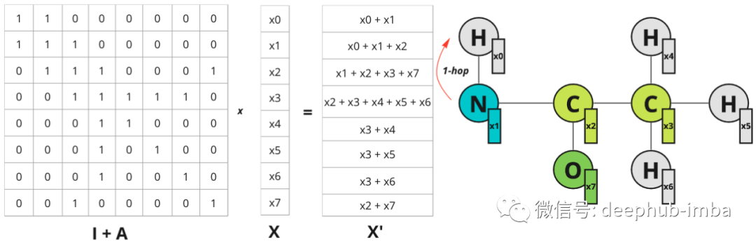
For each node, the sum of adjacent nodes is added. So the operation can be expressed as follows:

N(i) represents the one-hop distance neighbor of node i.

In this example, "update" and "aggregate" are simply summation functions.

This feature update on the node is called a message passing mechanism. A single iteration of such message passing is equivalent to graph convolution with filter P = I + A. Then if we want to propagate information from farther nodes, we can repeat this operation several times again, approximating the graph convolution with more polynomial terms.

One caveat though: if you repeat the graph convolution multiple times, you can cause the graph to be over-smoothed, where each node embedding becomes the same average vector for all connected nodes.

So how to enhance the expressiveness of message delivery? You can try aggregation and update functions, and additionally transform node features:

W1——Update the weight matrix of node features, W2——Update the weight matrix of adjacent node features.

Aggregations can be performed using any permutation-invariant function such as sum, max, mean or more complex functions such as DeepSets.

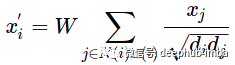
For example, one of the basic ways to evaluate message passing is the GCN layer:

This formula may not be familiar at first sight, but let's take a look at it using the "update" and "aggregate" functions:

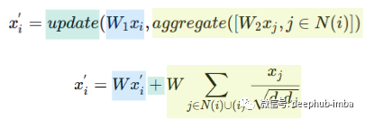
A single matrix W is used instead of the two weight matrices W1 and W2. The update function is the summation and the aggregation function is the sum of normalized node features, including node feature i. d - represents the node degree.

This uses one weight matrix W instead of two, and uses Kipf and Welling normalized summation as aggregation and a summation as update function. Aggregation operations evaluate neighbors and node i itself, which is equivalent to adding self-loops to the graph.

So GNN with message passing mechanism can be represented as multiple repeated aggregation and update functions. Each iteration of message passing can be viewed as a new GNN layer. All operations on node updates are differentiable and can be parameterized with a weight matrix that can be learned. Now we can build a graph convolutional network and explore how it performs.

a practical example

Build and train a graph neural network using the GCN layers mentioned above. For this example, I will use the PyG library and the AIDS graph dataset provided in [2]. It consists of 2000 graphs representing molecular compounds: 1600 of which are considered inactive against HIV and 400 of which are active against HIV. Each node has a feature vector with 38 features. Here is an example of a molecular graph representation in the dataset:

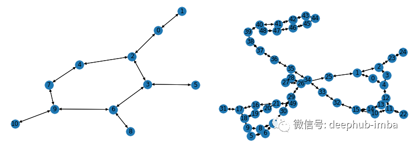
Visualize samples from the AIDS dataset using the networkx library.

For simplicity, we will build a model with only 3 GCN layers. The final embedding dimension for the visualization of the embedding space will be 2-d. To obtain graph embeddings, mean aggregation will be used. To classify the molecules, a simple linear classifier will be used after the graph embedding.

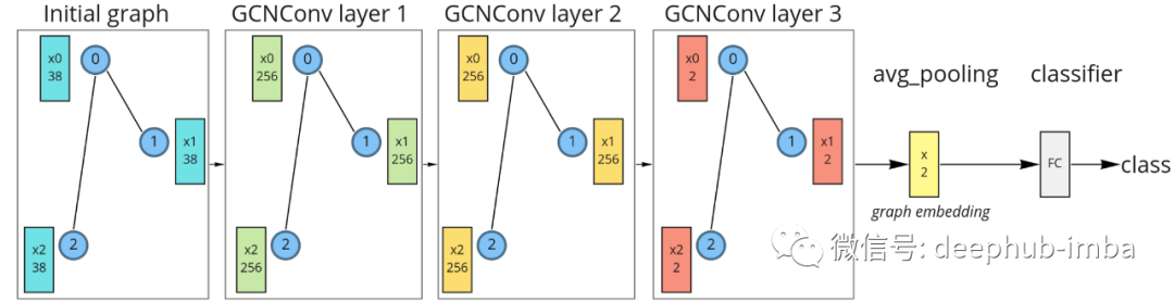
Graph neural network with three GCN layers, average pooling, and linear classifiers.

For the first iteration of message passing (layer 1), the initial feature vectors are projected into the 256-dimensional space. During the second message pass (layer 2), the feature vector is updated in the same dimension. During the third message pass (layer 3), the features are projected into a 2D space, and then all node features are averaged to obtain the final graph embedding. Finally, these embeddings are fed to a linear classifier. The 2D dimension was chosen just for visualization, higher dimensions would definitely be better. Such a model can be implemented using the PyG library:

from torch import nn
from torch.nn import functional as F
from torch_geometric.nn import GCNConv
from torch_geometric.nn import global_mean_pool


class GCNModel(nn.Module):
    def __init__(self, feature_node_dim=38, num_classes=2, hidden_dim=256, out_dim=2):
        super(GCNModel, self).__init__()
        torch.manual_seed(123)
        self.conv1 = GCNConv(feature_node_dim, hidden_dim)
        self.conv2 = GCNConv(hidden_dim, hidden_dim)
        self.conv3 = GCNConv(hidden_dim, out_dim)
        self.linear = nn.Linear(out_dim, num_classes)

    def forward(self, x, edge_index, batch):

        # Graph convolutions with nonlinearity:
        x = self.conv1(x, edge_index)
        x = F.relu(x)
        x = self.conv2(x, edge_index)
        x = F.relu(x)
        x = self.conv3(x, edge_index)

        # Graph embedding:
        x_embed = global_mean_pool(x, batch)

        # Linear classifier:
        x = self.linear(x_embed)

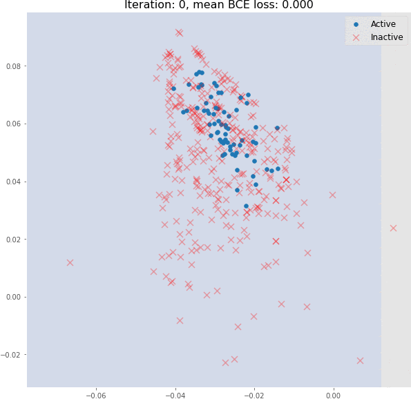
        return x, x_embed

During its training, graph embeddings and classifier decision boundaries can be visualized. You can see how the message passing operation enables the generation of meaningful graph embeddings using only 3 graph convolutional layers. The model embeddings using random initialization here do not have a linearly separable distribution:

The above figure is the molecular embedding obtained by forward propagation of the randomly initialized model

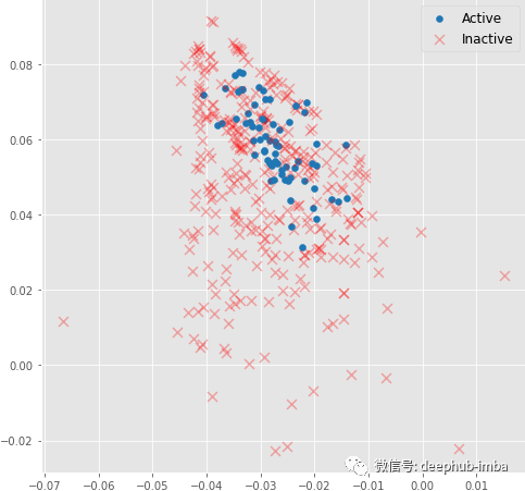
But during training, the molecular embedding quickly becomes linearly separable:

Even 3 graph convolutional layers can generate meaningful 2D molecular embeddings that can be classified using a linear model with ~82% accuracy on the validation set.

Summarize

In this paper, we describe how graph convolution is represented as a polynomial, and how it can be approximated using a message-passing mechanism. This method with additional feature transformations has powerful representation capabilities. This article has only scratched the surface of graph convolutions and graph neural networks. There are over a dozen different architectures for graph convolutional layers and aggregation functions. And there are many tasks that can be done on the graph, such as node classification, edge reconstruction, etc. So if you want to dig deeper, the PyG tutorial is a good place to start.

Author: Gleb Kumichev