1. math数学函数
1.1 特殊常量
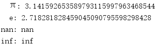
很多数学运算依赖于一些特殊的常量。math包含有π(pi)、e、nan(不是一个数)和infinity(无穷大)的值。
import math

print('  π: {:.30f}'.format(math.pi))
print('  e: {:.30f}'.format(math.e))
print('nan: {:.30f}'.format(math.nan))
print('inf: {:.30f}'.format(math.inf))
π和e的精度仅受平台的浮点数C库限制。
1.2 测试异常值
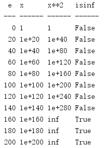
浮点数计算可能导致两种类型的异常值。第一种是inf(无穷大),当用double存储一个浮点数,而该值会从一个具体很大绝对值的值上溢出时,就会出现这个异常值。
import math

print('{:^3} {:6} {:6} {:6}'.format(
    'e', 'x', 'x**2', 'isinf'))
print('{:-^3} {:-^6} {:-^6} {:-^6}'.format(
    '', '', '', ''))

for e in range(0, 201, 20):
    x = 10.0 ** e
    y = x * x
    print('{:3d} {:<6g} {:<6g} {!s:6}'.format(
        e, x, y, math.isinf(y),
    ))
当这个例子中的指数变得足够大时,x的平方无法再存放一个double中,这个值就会被记录为无穷大。
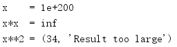
不过,并不是所有浮点数溢出都会导致inf值。具体地,用浮点值计算一个指数时,会产生OverflowError而不是保留inf结果。
x = 10.0 ** 200

print('x    =', x)
print('x*x  =', x * x)
print('x**2 =', end=' ')
try:
    print(x ** 2)
except OverflowError as err:
    print(err)
这种差异是由C和Python所用库中的实现差异造成的。
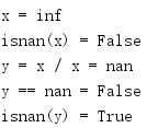
使用无穷大值的除法运算未定义。将一个数除以无穷大值的结果是nan(不是一个数)。
import math

x = (10.0 ** 200) * (10.0 ** 200)
y = x / x

print('x =', x)
print('isnan(x) =', math.isnan(x))
print('y = x / x =', x / x)
print('y == nan =', y == float('nan'))
print('isnan(y) =', math.isnan(y))
nan不等于任何值,甚至不等于其自身,所以要想检查nan,需要使用isnan()。
可以使用isfinite()检查其是普通的数还是特殊值inf或nan。
import math

for f in [0.0, 1.0, math.pi, math.e, math.inf, math.nan]:
    print('{:5.2f} {!s}'.format(f, math.isfinite(f)))
如果是特殊值inf或nan,则isfinite()返回false,否则返回true。

1.3 比较
涉及浮点值的比较容易出错,每一步计算都可能由于数值表示而引入误差,isclose()函数使用一种稳定的算法来尽可能减少这些误差,同时完成相对和绝对比较。所用的公式等价于:
abs(a-b) <= max(rel_tol * max(abs(a), abs(b)), abs_tol)
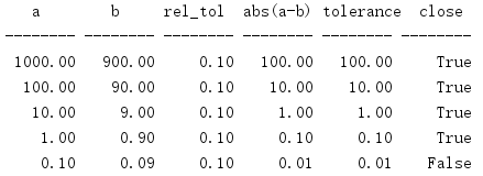
默认地,isclose()会完成相对比较,容差被设置为le-09,这表示两个值之差必须小于或等于le乘以a和b中较大的绝对值。向isclose()传入关键字参数rel_tol可以改变这个容差。在这个例子中,值之间的差距必须在10%以内。
import math

INPUTS = [
    (1000, 900, 0.1),
    (100, 90, 0.1),
    (10, 9, 0.1),
    (1, 0.9, 0.1),
    (0.1, 0.09, 0.1),
]

print('{:^8} {:^8} {:^8} {:^8} {:^8} {:^8}'.format(
    'a', 'b', 'rel_tol', 'abs(a-b)', 'tolerance', 'close')
)
print('{:-^8} {:-^8} {:-^8} {:-^8} {:-^8} {:-^8}'.format(
    '-', '-', '-', '-', '-', '-'),
)

fmt = '{:8.2f} {:8.2f} {:8.2f} {:8.2f} {:8.2f} {!s:>8}'

for a, b, rel_tol in INPUTS:
    close = math.isclose(a, b, rel_tol=rel_tol)
    tolerance = rel_tol * max(abs(a), abs(b))
    abs_diff = abs(a - b)
    print(fmt.format(a, b, rel_tol, abs_diff, tolerance, close))
0.1和0.09之间的比较失败,因为误差表示0.1。
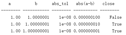
要使用一个固定或“绝对”容差,可以传入abs_tol而不是rel_tol。
import math

INPUTS = [
    (1.0, 1.0 + 1e-07, 1e-08),
    (1.0, 1.0 + 1e-08, 1e-08),
    (1.0, 1.0 + 1e-09, 1e-08),
]

print('{:^8} {:^11} {:^8} {:^10} {:^8}'.format(
    'a', 'b', 'abs_tol', 'abs(a-b)', 'close')
)
print('{:-^8} {:-^11} {:-^8} {:-^10} {:-^8}'.format(
    '-', '-', '-', '-', '-'),
)

for a, b, abs_tol in INPUTS:
    close = math.isclose(a, b, abs_tol=abs_tol)
    abs_diff = abs(a - b)
    print('{:8.2f} {:11} {:8} {:0.9f} {!s:>8}'.format(
        a, b, abs_tol, abs_diff, close))
对于绝对容差,输入值之差必须小于给定的容差。
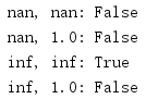
nan和inf是特殊情况。
import math

print('nan, nan:', math.isclose(math.nan, math.nan))
print('nan, 1.0:', math.isclose(math.nan, 1.0))
print('inf, inf:', math.isclose(math.inf, math.inf))
print('inf, 1.0:', math.isclose(math.inf, 1.0))
nan不接近任何值,包括它自身。inf只接近它自身。
1.4 将浮点值转换为整数
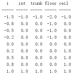
math模块中有3个函数用于将浮点值转换为整数。这3个函数分别采用不同的方法,并适用于不同的场合。
最简单的是trunc(),其会截断小数点后的数字,只留下构成这个值整数部分的有效数字。floor()将其输入转换为不大于它的最大整数,ceil()(上限)会生成按顺序排在这个输入值之后的最小整数。
import math

HEADINGS = ('i', 'int', 'trunk', 'floor', 'ceil')
print('{:^5} {:^5} {:^5} {:^5} {:^5}'.format(*HEADINGS))
print('{:-^5} {:-^5} {:-^5} {:-^5} {:-^5}'.format(
    '', '', '', '', '',
))

fmt = '{:5.1f} {:5.1f} {:5.1f} {:5.1f} {:5.1f}'

TEST_VALUES = [
    -1.5,
    -0.8,
    -0.5,
    -0.2,
    0,
    0.2,
    0.5,
    0.8,
    1,
]

for i in TEST_VALUES:
    print(fmt.format(
        i,
        int(i),
        math.trunc(i),
        math.floor(i),
        math.ceil(i),
    ))
trunc()等价于直接转换为int。
1.5 浮点值的其他表示
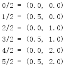
modf()取一个浮点数,并返回一个元组,其中包含这个输入值的小数和整数部分。
import math

for i in range(6):
    print('{}/2 = {}'.format(i, math.modf(i / 2.0)))
返回值中的两个数字均为浮点数。
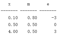
frexp()返回一个浮点数的尾数和指数,可以用这个函数创建值的一种更可移植的表示。
import math

print('{:^7} {:^7} {:^7}'.format('x', 'm', 'e'))
print('{:-^7} {:-^7} {:-^7}'.format('', '', ''))

for x in [0.1, 0.5, 4.0]:
    m, e = math.frexp(x)
    print('{:7.2f} {:7.2f} {:7d}'.format(x, m, e))
frexp()使用公式x = m * 2**e,并返回值m和e。
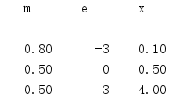
ldexp()与frexp()正好相反。
import math

print('{:^7} {:^7} {:^7}'.format('m', 'e', 'x'))
print('{:-^7} {:-^7} {:-^7}'.format('', '', ''))

INPUTS = [
    (0.8, -3),
    (0.5, 0),
    (0.5, 3),
]

for m, e in INPUTS:
    x = math.ldexp(m, e)
    print('{:7.2f} {:7d} {:7.2f}'.format(m, e, x))
ldexp()使用与frexp()相同的公式,取尾数和指数值作为参数,并返回一个浮点数。
1.6 正号和负号
一个数的绝对值就是不带正负号的本值。使用fabs()可以计算一个浮点数的绝对值。
import math

print(math.fabs(-1.1))
print(math.fabs(-0.0))
print(math.fabs(0.0))
print(math.fabs(1.1))
在实际中,float的绝对值表示为一个正值。

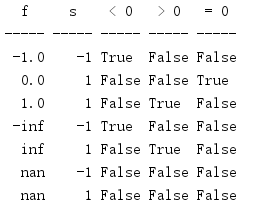
要确定一个值的符号,以便为一组值指定相同的符号或者比较两个值,可以使用copysign()来设置正确值的符号。
import math

HEADINGS = ('f', 's', '< 0', '> 0', '= 0')
print('{:^5} {:^5} {:^5} {:^5} {:^5}'.format(*HEADINGS))
print('{:-^5} {:-^5} {:-^5} {:-^5} {:-^5}'.format(
    '', '', '', '', '',
))

VALUES = [
    -1.0,
    0.0,
    1.0,
    float('-inf'),
    float('inf'),
    float('-nan'),
    float('nan'),
]

for f in VALUES:
    s = int(math.copysign(1, f))
    print('{:5.1f} {:5d} {!s:5} {!s:5} {!s:5}'.format(
        f, s, f < 0, f > 0, f == 0,
    ))
还需要另一个类似copysign()的函数,因为不能将nan和-nan与其他值直接比较。
1.7 常用计算
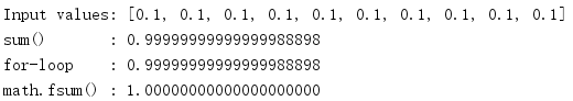
在二进制浮点数内存中表示精确度很有难度。有些值无法准确地表示,而且如果通过反复计算来处理一个值,那么计算越频繁就越容易引人表示误差。math包含一个函数来计算一系列浮点数的和,它使用一种高效的算法来尽量减少这种误差。
import math

values = [0.1] * 10

print('Input values:', values)

print('sum()       : {:.20f}'.format(sum(values)))

s = 0.0
for i in values:
    s += i
print('for-loop    : {:.20f}'.format(s))

print('math.fsum() : {:.20f}'.format(math.fsum(values)))
给定一个包含10个值的序列,每个值都等于0.1,这个序列总和的期望值为1.0。不过,由于0.1不能精确地表示为一个浮点数,所以会在总和中引入误差,除非用fsum()来计算。
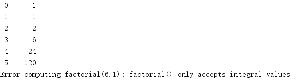
factorial()常用于计算一系列对象的排列和组合数。一个正整数n的阶乘(表示为n!)被递归的定义为(n-1)!*n,并在0!==1停止递归。
import math

for i in [0, 1.0, 2.0, 3.0, 4.0, 5.0, 6.1]:
    try:
        print('{:2.0f} {:6.0f}'.format(i, math.factorial(i)))
    except ValueError as err:
        print('Error computing factorial({}): {}'.format(i, err))
factorial()只能处理整数,不过它确实也接受float参数,只要这个参数可以转换为一个整数而不丢值。
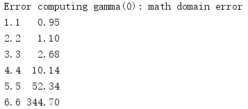
gamma()类似于factorial(),不过它可以处理实数,而且值会下移一个数(gamma等于(n - 1)!)。
import math

for i in [0, 1.1, 2.2, 3.3, 4.4, 5.5, 6.6]:
    try:
        print('{:2.1f} {:6.2f}'.format(i, math.gamma(i)))
    except ValueError as err:
        print('Error computing gamma({}): {}'.format(i, err))
由于0会导致开始值为负,所以这是不允许的。
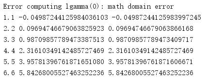
lgamma()会返回对输入值求gamma所得结果的绝对值的自然对数。
import math

for i in [0, 1.1, 2.2, 3.3, 4.4, 5.5, 6.6]:
    try:
        print('{:2.1f} {:.20f} {:.20f}'.format(
            i,
            math.lgamma(i),
            math.log(math.gamma(i)),
        ))
    except ValueError as err:
        print('Error computing lgamma({}): {}'.format(i, err))
使用lgamma()会比使用gamma()结果单独计算对数更精确。
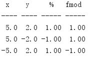
求模操作符(%)会计算一个除法表达式的余数(例如,5 % 2 = 1)。Python语言内置的这个操作符可以很好地处理整数,但是与很多其他浮点数运算类似,中间计算可能带来表示问题,从而进一步造成数据丢失。fmod()可以为浮点值提供一个更精确的实现。
import math

print('{:^4} {:^4} {:^5} {:^5}'.format(
    'x', 'y', '%', 'fmod'))
print('{:-^4} {:-^4} {:-^5} {:-^5}'.format(
    '-', '-', '-', '-'))

INPUTS = [
    (5, 2),
    (5, -2),
    (-5, 2),
]

for x, y in INPUTS:
    print('{:4.1f} {:4.1f} {:5.2f} {:5.2f}'.format(
        x,
        y,
        x % y,
        math.fmod(x, y),
    ))
还有一点可能经常产生混淆,即fmod()计算模所使用的算法与%使用的算法也有所不同,所以结果的符号不同。
可以使用gcd()找出两个整数公约数中最大的整数——也就是最大公约数。
import math

print(math.gcd(10, 8))
print(math.gcd(10, 0))
print(math.gcd(50, 225))
print(math.gcd(11, 9))
print(math.gcd(0, 0))
如果两个值都为0,则结果为0。

1.8 指数和对数
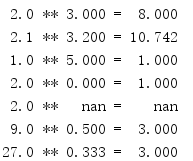
指数生长曲线在经济学、物理学和其他科学中经常出现。Python有一个内置的幂运算符(“**”),不过,如果需要将一个可调用函数作为另一个函数的参数,那么可能需要用到pow()。
import math

INPUTS = [
    # Typical uses
    (2, 3),
    (2.1, 3.2),

    # Always 1
    (1.0, 5),
    (2.0, 0),

    # Not-a-number
    (2, float('nan')),

    # Roots
    (9.0, 0.5),
    (27.0, 1.0 / 3),
]

for x, y in INPUTS:
    print('{:5.1f} ** {:5.3f} = {:6.3f}'.format(
        x, y, math.pow(x, y)))
1的任何次幂总返回1.0,同样,任何值的指数为0.0时也总是返回1.0.对于nan值(不是一个数),大多数运算都返回nan。如果指数小于1,pow()会计算一个根。
由于平方根(指数为1/2)被使用的非常频繁,所以有一个单独的函数来计算平方根。
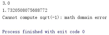
import math

print(math.sqrt(9.0))
print(math.sqrt(3))
try:
    print(math.sqrt(-1))
except ValueError as err:
    print('Cannot compute sqrt(-1):', err)
计算负数的平方根需要用到复数,这不在math的处理范围内。试图计算一个负值的平方根时,会导致一个ValueError。
对数函数查找满足条件x=b**y的y。默认log()计算自然对数(底数为e)。如果提供了第二个参数,则使用这个参数值作为底数。
import math

print(math.log(8))
print(math.log(8, 2))
print(math.log(0.5, 2))
x小于1时,求对数会产生负数结果。

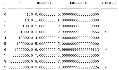
log()有三个变形。在给定浮点数表示和取整误差的情况下,由log(x,b)生成的计算值只有有限的精度(特别是对于某些底数)。log10()完成log(x,10)计算,但是会使用一种比log()更精确的算法。
import math

print('{:2} {:^12} {:^10} {:^20} {:8}'.format(
    'i', 'x', 'accurate', 'inaccurate', 'mismatch',
))
print('{:-^2} {:-^12} {:-^10} {:-^20} {:-^8}'.format(
    '', '', '', '', '',
))

for i in range(0, 10):
    x = math.pow(10, i)
    accurate = math.log10(x)
    inaccurate = math.log(x, 10)
    match = '' if int(inaccurate) == i else '*'
    print('{:2d} {:12.1f} {:10.8f} {:20.18f} {:^5}'.format(
        i, x, accurate, inaccurate, match,
    ))
输出中末尾有*的行突出强调了不精确的值。
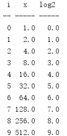
类似于log10(),log2()会完成等价于math.log(x,2)的计算。
import math

print('{:>2} {:^5} {:^5}'.format(
    'i', 'x', 'log2',
))
print('{:-^2} {:-^5} {:-^5}'.format(
    '', '', '',
))

for i in range(0, 10):
    x = math.pow(2, i)
    result = math.log2(x)
    print('{:2d} {:5.1f} {:5.1f}'.format(
        i, x, result,
    ))
取决于底层平台,这个内置的特殊用途函数能提供更好的性能和精度,因为它利用了针对底数2的特殊用途算法,而在更一般用途的函数中没有使用这些算法。
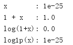
log1p()会计算Newton-Mercator序列(1+x的自然对数)。
import math

x = 0.0000000000000000000000001
print('x       :', x)
print('1 + x   :', 1 + x)
print('log(1+x):', math.log(1 + x))
print('log1p(x):', math.log1p(x))
对于非常接近于0的x,log1p()会更为精确,因为它使用的算法可以补偿由初识加法带来的取整误差。
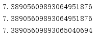
exp()会计算指数函数(e**x)。
import math

x = 2

fmt = '{:.20f}'
print(fmt.format(math.e ** 2))
print(fmt.format(math.pow(math.e, 2)))
print(fmt.format(math.exp(2)))
类似于其他特殊函数,与等价的通用函数math.pow(math.e,x)相比,exp()使用的算法可以生成更精确的结果。
expm1()是log1p()的逆运算,会计算e**x-1。
import math

x = 0.0000000000000000000000001

print(x)
print(math.exp(x) - 1)
print(math.expm1(x))
类似于log1p(),x值很小时,如果单独完成减法,则可能会损失精度。

1.9 角
尽管我们每天讨论角时更常用的是度,但弧度才是科学和数学领域中度量角度的标准单位。弧度是在圆心相交的两条线所构成的角,其终点落在圆的圆周上,终点之间相距一个弧度。
圆周长计算为2πr,所以弧度与π(这是三角函数计算中经常出现的一个值)之间存在一个关系。这个关系使得三角学和微积分中都使用了弧度,因为利用弧度可以得到更紧凑的公式。
要把度转换为弧度,可以使用redians()。
import math

print('{:^7} {:^7} {:^7}'.format(
    'Degrees', 'Radians', 'Expected'))
print('{:-^7} {:-^7} {:-^7}'.format(
    '', '', ''))

INPUTS = [
    (0, 0),
    (30, math.pi / 6),
    (45, math.pi / 4),
    (60, math.pi / 3),
    (90, math.pi / 2),
    (180, math.pi),
    (270, 3 / 2.0 * math.pi),
    (360, 2 * math.pi),
]

for deg, expected in INPUTS:
    print('{:7d} {:7.2f} {:7.2f}'.format(
        deg,
        math.radians(deg),
        expected,
    ))
转换公式为rad = deg * π / 180。

要从弧度转换为度,可以使用degrees()。
import math

INPUTS = [
    (0, 0),
    (math.pi / 6, 30),
    (math.pi / 4, 45),
    (math.pi / 3, 60),
    (math.pi / 2, 90),
    (math.pi, 180),
    (3 * math.pi / 2, 270),
    (2 * math.pi, 360),
]

print('{:^8} {:^8} {:^8}'.format(
    'Radians', 'Degrees', 'Expected'))
print('{:-^8} {:-^8} {:-^8}'.format('', '', ''))
for rad, expected in INPUTS:
    print('{:8.2f} {:8.2f} {:8.2f}'.format(
        rad,
        math.degrees(rad),
        expected,
    ))
具体转换公式为deg = rad * 180 / π。

1.10 三角函数
三角函数将三角形中的角与其边长相关联。在有周期性质的公式中经常出现三角函数,如谐波或圆周运动;在处理角时也会经常用到三角函数。标准库中所有三角函数的角参数都被表示为弧度。
给定一个直角三角形中的角,其正弦是对边长度与斜边长度之比(sin A = 对边/斜边)。余弦是邻边长度与斜边长度之比(cos A = 邻边/斜边)。正切是对边与邻边之比(tan A = 对边/邻边)。
import math

print('{:^7} {:^7} {:^7} {:^7} {:^7}'.format(
    'Degrees', 'Radians', 'Sine', 'Cosine', 'Tangent'))
print('{:-^7} {:-^7} {:-^7} {:-^7} {:-^7}'.format(
    '-', '-', '-', '-', '-'))

fmt = '{:7.2f} {:7.2f} {:7.2f} {:7.2f} {:7.2f}'

for deg in range(0, 361, 30):
    rad = math.radians(deg)
    if deg in (90, 270):
        t = float('inf')
    else:
        t = math.tan(rad)
    print(fmt.format(deg, rad, math.sin(rad), math.cos(rad), t))
正切也可以被定义为角的正弦值与其余弦值之比,因为弧度π/2和3π/2的余弦是0,所以相应的正切值为无穷大。

给定一个点(x,y),点[(0,0),(x,0),(x,y)]构成的三角形中斜边长度为(x**2+y**2)**1/2,可以用hypot()来计算。
import math

print('{:^7} {:^7} {:^10}'.format('X', 'Y', 'Hypotenuse'))
print('{:-^7} {:-^7} {:-^10}'.format('', '', ''))

POINTS = [
    # simple points
    (1, 1),
    (-1, -1),
    (math.sqrt(2), math.sqrt(2)),
    (3, 4),  # 3-4-5 triangle
    # on the circle
    (math.sqrt(2) / 2, math.sqrt(2) / 2),  # pi/4 rads
    (0.5, math.sqrt(3) / 2),  # pi/3 rads
]

for x, y in POINTS:
    h = math.hypot(x, y)
    print('{:7.2f} {:7.2f} {:7.2f}'.format(x, y, h))
对于圆上的点,其斜边总是等于1。

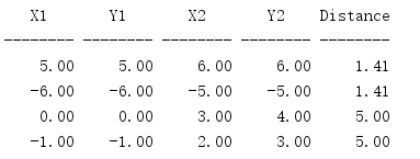
还可以用这个函数查看两个点之间的距离。
import math

print('{:^8} {:^8} {:^8} {:^8} {:^8}'.format(
    'X1', 'Y1', 'X2', 'Y2', 'Distance',
))
print('{:-^8} {:-^8} {:-^8} {:-^8} {:-^8}'.format(
    '', '', '', '', '',
))

POINTS = [
    ((5, 5), (6, 6)),
    ((-6, -6), (-5, -5)),
    ((0, 0), (3, 4)),  # 3-4-5 triangle
    ((-1, -1), (2, 3)),  # 3-4-5 triangle
]

for (x1, y1), (x2, y2) in POINTS:
    x = x1 - x2
    y = y1 - y2
    h = math.hypot(x, y)
    print('{:8.2f} {:8.2f} {:8.2f} {:8.2f} {:8.2f}'.format(
        x1, y1, x2, y2, h,
    ))
使用x值之差和y值之差将一个端点移至原点,然后将结果传入hypot()。
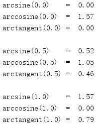
math还定义了反三角函数。
import math

for r in [0, 0.5, 1]:
    print('arcsine({:.1f})    = {:5.2f}'.format(r, math.asin(r)))
    print('arccosine({:.1f})  = {:5.2f}'.format(r, math.acos(r)))
    print('arctangent({:.1f}) = {:5.2f}'.format(r, math.atan(r)))
    print()
1.57大约对于π/2,或90度,这个角的正弦为1,余弦为0。
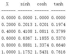
1.11 双曲函数
双曲函数经常出现在线性微分方程中,处理电磁场、流体力学、狭义相对论和其他高级物理和数学问题时常会用到。
import math

print('{:^6} {:^6} {:^6} {:^6}'.format(
    'X', 'sinh', 'cosh', 'tanh',
))
print('{:-^6} {:-^6} {:-^6} {:-^6}'.format('', '', '', ''))

fmt = '{:6.4f} {:6.4f} {:6.4f} {:6.4f}'

for i in range(0, 11, 2):
    x = i / 10.0
    print(fmt.format(
        x,
        math.sinh(x),
        math.cosh(x),
        math.tanh(x),
    ))
余弦函数和正弦函数构成一个圆,而双曲余弦函数和双曲正弦函数构成半个双曲线。
另外还提供了反双曲函数acosh()、asinh()和atanh()。
1.12 特殊函数
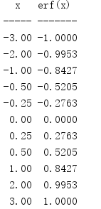
统计学中经常用到高斯误差函数(Gauss error function)。
import math

print('{:^5} {:7}'.format('x', 'erf(x)'))
print('{:-^5} {:-^7}'.format('', ''))

for x in [-3, -2, -1, -0.5, -0.25, 0, 0.25, 0.5, 1, 2, 3]:
    print('{:5.2f} {:7.4f}'.format(x, math.erf(x)))
对于误差函数,erf(-x) == -erf(x)。
补余误差函数erfc()生成等价于1 - erf(x)的值。
import math

print('{:^5} {:7}'.format('x', 'erfc(x)'))
print('{:-^5} {:-^7}'.format('', ''))

for x in [-3, -2, -1, -0.5, -0.25, 0, 0.25, 0.5, 1, 2, 3]:
    print('{:5.2f} {:7.4f}'.format(x, math.erfc(x)))
如果x值很小,那么在从1做减法时erfc()实现便可以避免可能的精度误差。
