1、说明
最近,做因子回测时用到了Alphalens,这里简单介绍下alphalens的使用,但是由于有一篇东北证券的研报写得还算清楚了,而且由于是开源的,大家可以直接看源代码,那篇研报基本上也就是翻译了一下源代码的介绍而已,在这里的话,建议大家可以看一眼研报,然后使用前,还是看一下源码,可能是因为后来alphalens又更新了,那篇研报上有一些函数的参数有错误。
本篇博文会简单介绍下alphalens的使用,但是介绍不作重点,主要还是记录下使用过程中的一些坑。
2、数据预处理:get_clean_factor_and_forward_returns
alphalens里最重要的应该就是整理好源数据了,get_clean_factor_and_forward_returns就是整理源数据的函数,只要完成这步骤,所有技术性的工作就都结束了,后面主要就是解读结果,当然解读结果也是挺费劲的,我也看了好久的源码,后面再说。
get_clean_factor_and_forward_returns使用介绍
这个函数是在utils.py文件中的,先贴一段源码:
def get_clean_factor_and_forward_returns(factor,
                                         prices,
                                         groupby=None,
                                         binning_by_group=False,
                                         quantiles=5,
                                         bins=None,
                                         periods=(1, 5, 10),
                                         filter_zscore=20,
                                         groupby_labels=None,
                                         max_loss=0.35,
                                         zero_aware=False,
                                         cumulative_returns=True):
    """
    Formats the factor data, pricing data, and group mappings into a DataFrame
    that contains aligned MultiIndex indices of timestamp and asset. The
    returned data will be formatted to be suitable for Alphalens functions.

    It is safe to skip a call to this function and still make use of Alphalens
    functionalities as long as the factor data conforms to the format returned
    from get_clean_factor_and_forward_returns and documented here

    Parameters
    ----------
    factor : pd.Series - MultiIndex
        A MultiIndex Series indexed by timestamp (level 0) and asset
        (level 1), containing the values for a single alpha factor.
        ::
            -----------------------------------
                date    |    asset   |
            -----------------------------------
                        |   AAPL     |   0.5
                        -----------------------
                        |   BA       |  -1.1
                        -----------------------
            2014-01-01  |   CMG      |   1.7
                        -----------------------
                        |   DAL      |  -0.1
                        -----------------------
                        |   LULU     |   2.7
                        -----------------------

    prices : pd.DataFrame
        A wide form Pandas DataFrame indexed by timestamp with assets
        in the columns.
        Pricing data must span the factor analysis time period plus an
        additional buffer window that is greater than the maximum number
        of expected periods in the forward returns calculations.
        It is important to pass the correct pricing data in depending on
        what time of period your signal was generated so to avoid lookahead
        bias, or  delayed calculations.
        'Prices' must contain at least an entry for each timestamp/asset
        combination in 'factor'. This entry should reflect the buy price
        for the assets and usually it is the next available price after the
        factor is computed but it can also be a later price if the factor is
        meant to be traded later (e.g. if the factor is computed at market
        open but traded 1 hour after market open the price information should
        be 1 hour after market open).
        'Prices' must also contain entries for timestamps following each
        timestamp/asset combination in 'factor', as many more timestamps
        as the maximum value in 'periods'. The asset price after 'period'
        timestamps will be considered the sell price for that asset when
        computing 'period' forward returns.
        ::
            ----------------------------------------------------
                        | AAPL |  BA  |  CMG  |  DAL  |  LULU  |
            ----------------------------------------------------
               Date     |      |      |       |       |        |
            ----------------------------------------------------
            2014-01-01  |605.12| 24.58|  11.72| 54.43 |  37.14 |
            ----------------------------------------------------
            2014-01-02  |604.35| 22.23|  12.21| 52.78 |  33.63 |
            ----------------------------------------------------
            2014-01-03  |607.94| 21.68|  14.36| 53.94 |  29.37 |
            ----------------------------------------------------

    groupby : pd.Series - MultiIndex or dict
        Either A MultiIndex Series indexed by date and asset,
        containing the period wise group codes for each asset, or
        a dict of asset to group mappings. If a dict is passed,
        it is assumed that group mappings are unchanged for the
        entire time period of the passed factor data.
    binning_by_group : bool
        If True, compute quantile buckets separately for each group.
        This is useful when the factor values range vary considerably
        across gorups so that it is wise to make the binning group relative.
        You should probably enable this if the factor is intended
        to be analyzed for a group neutral portfolio
    quantiles : int or sequence[float]
        Number of equal-sized quantile buckets to use in factor bucketing.
        Alternately sequence of quantiles, allowing non-equal-sized buckets
        e.g. [0, .10, .5, .90, 1.] or [.05, .5, .95]
        Only one of 'quantiles' or 'bins' can be not-None
    bins : int or sequence[float]
        Number of equal-width (valuewise) bins to use in factor bucketing.
        Alternately sequence of bin edges allowing for non-uniform bin width
        e.g. [-4, -2, -0.5, 0, 10]
        Chooses the buckets to be evenly spaced according to the values
        themselves. Useful when the factor contains discrete values.
        Only one of 'quantiles' or 'bins' can be not-None
    periods : sequence[int]
        periods to compute forward returns on.
    filter_zscore : int or float, optional
        Sets forward returns greater than X standard deviations
        from the the mean to nan. Set it to 'None' to avoid filtering.
        Caution: this outlier filtering incorporates lookahead bias.
    groupby_labels : dict
        A dictionary keyed by group code with values corresponding
        to the display name for each group.
    max_loss : float, optional
        Maximum percentage (0.00 to 1.00) of factor data dropping allowed,
        computed comparing the number of items in the input factor index and
        the number of items in the output DataFrame index.
        Factor data can be partially dropped due to being flawed itself
        (e.g. NaNs), not having provided enough price data to compute
        forward returns for all factor values, or because it is not possible
        to perform binning.
        Set max_loss=0 to avoid Exceptions suppression.
    zero_aware : bool, optional
        If True, compute quantile buckets separately for positive and negative
        signal values. This is useful if your signal is centered and zero is
        the separation between long and short signals, respectively.
    cumulative_returns : bool, optional
        If True, forward returns columns will contain cumulative returns.
        Setting this to False is useful if you want to analyze how predictive
        a factor is for a single forward day.

    Returns
    -------
    merged_data : pd.DataFrame - MultiIndex
        A MultiIndex Series indexed by date (level 0) and asset (level 1),
        containing the values for a single alpha factor, forward returns for
        each period, the factor quantile/bin that factor value belongs to, and
        (optionally) the group the asset belongs to.
        - forward returns column names follow  the format accepted by
          pd.Timedelta (e.g. '1D', '30m', '3h15m', '1D1h', etc)
        - 'date' index freq property (merged_data.index.levels[0].freq) will be
          set to a trading calendar (pandas DateOffset) inferred from the input
          data (see infer_trading_calendar for more details). This is currently
          used only in cumulative returns computation
        ::
           -------------------------------------------------------------------
                      |       | 1D  | 5D  | 10D  |factor|group|factor_quantile
           -------------------------------------------------------------------
               date   | asset |     |     |      |      |     |
           -------------------------------------------------------------------
                      | AAPL  | 0.09|-0.01|-0.079|  0.5 |  G1 |      3
                      --------------------------------------------------------
                      | BA    | 0.02| 0.06| 0.020| -1.1 |  G2 |      5
                      --------------------------------------------------------
           2014-01-01 | CMG   | 0.03| 0.09| 0.036|  1.7 |  G2 |      1
                      --------------------------------------------------------
                      | DAL   |-0.02|-0.06|-0.029| -0.1 |  G3 |      5
                      --------------------------------------------------------
                      | LULU  |-0.03| 0.05|-0.009|  2.7 |  G1 |      2
                      --------------------------------------------------------
    """

    forward_returns = compute_forward_returns(factor, prices, periods,
                                              filter_zscore,
                                              cumulative_returns)

    factor_data = get_clean_factor(factor, forward_returns, groupby=groupby,
                                   groupby_labels=groupby_labels,
                                   quantiles=quantiles, bins=bins,
                                   binning_by_group=binning_by_group,
                                   max_loss=max_loss, zero_aware=zero_aware)

    return factor_data
具体的输入源码里写的非常清楚了,这里写几个注意的点:
- 第一个参数factor为时间作为第一索引,股票代码作为第二索引的series,这边的factor一般是需要每天的factor,因为后面的prices一般是每天的股价,这两个参数的数据必须是一一对应的,我建议可以先把factor和股价整理到一个dataframe中,然后按照这个函数的要求从一个统一的dataframe中拆出来,这样就不会出问题了。
- 第二个参数是每天的股价的数据,这个参数在时间上需要与第一个参数对应,使用我上述说的从一个dataframe中拆出来就不会出现问题。
- 如果说前面两者参数中缺失值过多,则max_loss这个参数可以适当调到一些,因为这个函数在整理数据的过程中会将factor中NAN的值全部删掉,并且会记录删除的数据的百分比,如果之前的数据中缺失值过多,那么删除掉的百分比就会过大,造成报错。
- 前面提到的factor和price需要每天的数据也不是一定的,有一次我就使用了一季度一个数据,factor和price都是一季度一个,也是可以成功运行的,跑出来的结果也可以分析,但是不建议这样,因为这会导致之后绘制出的收益累计图等很奇怪,不大正常,当然如果这样做了,分析也没问题。
- 很多时候可能都是一季度一个数据(季报数据),那么如何将其变成每天都有数据呢?只需要将一季度一个的factor和每天都有的price做右连接,这样就得到了一个每天都有price和factor,当然绝大多数天数的factor是空的,这时使用dataframe.fillna(method = ‘ffill’)就行了,也就是向后填充,即在季报公布后,则使用这个数据直到下一份季报数据公布。
- 这里要特别强调一下periods这个参数,之前我一直把这个periods当做是调仓周期,其实不是的,这个应该是理解成持有周期,因为文档对periods的解释是:*periods : sequence[int]:periods to compute forward returns on.*计算收益的周期,也就意味着是你持有的时间,那问题来了,换仓周期要怎么设置呢?其实换仓周期是不用设置的,你传进来的factor这个参数就告诉我们你的换仓周期了,因为factor的计算周期也就是换仓周期,Quanlens是在根据factor来计算分组收益以及因子加权、多空等收益的,所以factor不变就意味着是不调仓,factor变了,就意味着factor分组变了,也就是说调仓了!
总的来说,我使用的整理方法如下:
- 读取季报数据,计算因子值,存到df_factor;
- 读取每天的收盘价数据,存到df_price;
- df_merge = pd.merge(df_price , df_factor[[‘Accper’ , ‘StockCode’ , ‘factor’]] , on = [‘StockCode’ , ‘Accper’] , how = ‘left’)
- for stock in stock_list:
df_temp[‘factor’] = df_temp[[‘factor’]].fillna(method = ‘ffill’)
df_final = pd.concat(df_final , df_temp)
end for - df_final就是最终需要的dataframe,之后可以利用该datafranme得到所需的get_clean_factor_and_forward_returns函数的第一二个参数。
3、因子IC分析
这是分析因子和收益间的相关性的,也就是因子的有效性和稳定性,有了前面函数得到的返回值df_alpha后就很简单了,直接调用函数就行了。
该函数在tears.py中的,源码如下:
@plotting.customize
def create_information_tear_sheet(factor_data,
                                  group_neutral=False,
                                  by_group=False):
    """
    Creates a tear sheet for information analysis of a factor.

    Parameters
    ----------
    factor_data : pd.DataFrame - MultiIndex
        A MultiIndex DataFrame indexed by date (level 0) and asset (level 1),
        containing the values for a single alpha factor, forward returns for
        each period, the factor quantile/bin that factor value belongs to, and
        (optionally) the group the asset belongs to.
        - See full explanation in utils.get_clean_factor_and_forward_returns
    group_neutral : bool
        Demean forward returns by group before computing IC.
    by_group : bool
        If True, display graphs separately for each group.
    """

    ic = perf.factor_information_coefficient(factor_data, group_neutral)

    plotting.plot_information_table(ic)

    columns_wide = 2
    fr_cols = len(ic.columns)
    rows_when_wide = (((fr_cols - 1) // columns_wide) + 1)
    vertical_sections = fr_cols + 3 * rows_when_wide + 2 * fr_cols
    gf = GridFigure(rows=vertical_sections, cols=columns_wide)

    ax_ic_ts = [gf.next_row() for _ in range(fr_cols)]
    plotting.plot_ic_ts(ic, ax=ax_ic_ts)

    ax_ic_hqq = [gf.next_cell() for _ in range(fr_cols * 2)]
    plotting.plot_ic_hist(ic, ax=ax_ic_hqq[::2])
    plotting.plot_ic_qq(ic, ax=ax_ic_hqq[1::2])

    if not by_group:

        mean_monthly_ic = \
            perf.mean_information_coefficient(factor_data,
                                              group_adjust=group_neutral,
                                              by_group=False,
                                              by_time="M")
        ax_monthly_ic_heatmap = [gf.next_cell() for x in range(fr_cols)]
        plotting.plot_monthly_ic_heatmap(mean_monthly_ic,
                                         ax=ax_monthly_ic_heatmap)

    if by_group:
        mean_group_ic = \
            perf.mean_information_coefficient(factor_data,
                                              group_adjust=group_neutral,
                                              by_group=True)

        plotting.plot_ic_by_group(mean_group_ic, ax=gf.next_row())

    plt.show()
    gf.close()
该函数返回两个东西,1、因子IC信息表;2、因子IC信息图
分别如下所示:
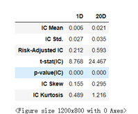
IC mean就是所有IC值的均值,IC std就是所有IC值的标准差,还有t统计量,p值和峰度偏度值。
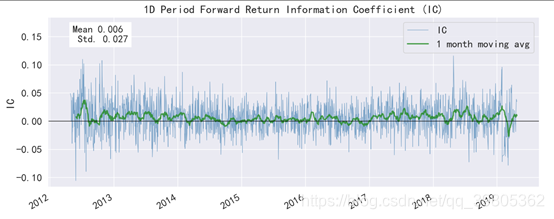
IC值随时间变化值,大部分都是大于0,可见大部分时候该因子和下期收益都是正相关的。
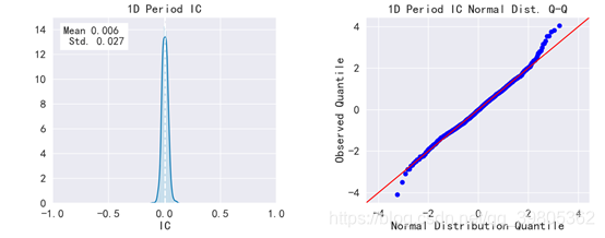
该图是IC分布,和QQ图,该图显示IC是标准正态分布的
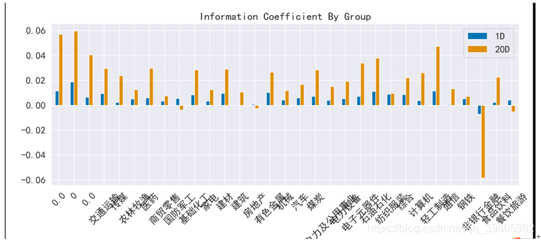
各个行业的IC值信息
这个函数的结果很清晰,也很容易理解
4、因子收益分析
create_returns_tear_sheet函数可以得到收益情况,下面是源码:
只有 long_short参数需要注意一下,该参数为True,则计算收益时会进行demean(中心化)操作,绘制的图也是demean后的,详见后面的结果。其余就没什么要讲的了。
@plotting.customize
def create_returns_tear_sheet(factor_data,
                              long_short=True,
                              group_neutral=False,
                              by_group=False):
    """
    Creates a tear sheet for returns analysis of a factor.

    Parameters
    ----------
    factor_data : pd.DataFrame - MultiIndex
        A MultiIndex DataFrame indexed by date (level 0) and asset (level 1),
        containing the values for a single alpha factor, forward returns for
        each period, the factor quantile/bin that factor value belongs to,
        and (optionally) the group the asset belongs to.
        - See full explanation in utils.get_clean_factor_and_forward_returns
    long_short : bool
        Should this computation happen on a long short portfolio? if so, then
        mean quantile returns will be demeaned across the factor universe.
        Additionally factor values will be demeaned across the factor universe
        when factor weighting the portfolio for cumulative returns plots
    group_neutral : bool
        Should this computation happen on a group neutral portfolio? if so,
        returns demeaning will occur on the group level.
        Additionally each group will weight the same in cumulative returns
        plots
    by_group : bool
        If True, display graphs separately for each group.
    """

    factor_returns = perf.factor_returns(factor_data,
                                         long_short,
                                         group_neutral)

    mean_quant_ret, std_quantile = \
        perf.mean_return_by_quantile(factor_data,
                                     by_group=False,
                                     demeaned=long_short,
                                     group_adjust=group_neutral)

    mean_quant_rateret = \
        mean_quant_ret.apply(utils.rate_of_return, axis=0,
                             base_period=mean_quant_ret.columns[0])

    mean_quant_ret_bydate, std_quant_daily = \
        perf.mean_return_by_quantile(factor_data,
                                     by_date=True,
                                     by_group=False,
                                     demeaned=long_short,
                                     group_adjust=group_neutral)

    mean_quant_rateret_bydate = mean_quant_ret_bydate.apply(
        utils.rate_of_return, axis=0,
        base_period=mean_quant_ret_bydate.columns[0]
    )

    compstd_quant_daily = \
        std_quant_daily.apply(utils.std_conversion, axis=0,
                              base_period=std_quant_daily.columns[0])

    alpha_beta = perf.factor_alpha_beta(factor_data,
                                        factor_returns,
                                        long_short,
                                        group_neutral)

    mean_ret_spread_quant, std_spread_quant = \
        perf.compute_mean_returns_spread(mean_quant_rateret_bydate,
                                         factor_data['factor_quantile'].max(),
                                         factor_data['factor_quantile'].min(),
                                         std_err=compstd_quant_daily)

    fr_cols = len(factor_returns.columns)
    vertical_sections = 2 + fr_cols * 3
    gf = GridFigure(rows=vertical_sections, cols=1)

    plotting.plot_returns_table(alpha_beta,
                                mean_quant_rateret,
                                mean_ret_spread_quant)

    plotting.plot_quantile_returns_bar(mean_quant_rateret,
                                       by_group=False,
                                       ylim_percentiles=None,
                                       ax=gf.next_row())

    plotting.plot_quantile_returns_violin(mean_quant_rateret_bydate,
                                          ylim_percentiles=(1, 99),
                                          ax=gf.next_row())

    trading_calendar = factor_data.index.levels[0].freq
    if trading_calendar is None:
        trading_calendar = pd.tseries.offsets.BDay()
        warnings.warn(
            "'freq' not set in factor_data index: assuming business day",
            UserWarning
        )

    for p in factor_returns:

        title = ('Factor Weighted '
                 + ('Group Neutral ' if group_neutral else '')
                 + ('Long/Short ' if long_short else '')
                 + "Portfolio Cumulative Return ({} Period)".format(p))

        plotting.plot_cumulative_returns(
            factor_returns[p],
            period=p,
            freq=trading_calendar,
            title=title,
            ax=gf.next_row()
        )

        plotting.plot_cumulative_returns_by_quantile(
            mean_quant_ret_bydate[p],
            period=p,
            freq=trading_calendar,
            ax=gf.next_row()
        )

    ax_mean_quantile_returns_spread_ts = [gf.next_row()
                                          for x in range(fr_cols)]
    plotting.plot_mean_quantile_returns_spread_time_series(
        mean_ret_spread_quant,
        std_err=std_spread_quant,
        bandwidth=0.5,
        ax=ax_mean_quantile_returns_spread_ts
    )

    plt.show()
    gf.close()

    if by_group:
        mean_return_quantile_group, mean_return_quantile_group_std_err = \
            perf.mean_return_by_quantile(factor_data,
                                         by_date=False,
                                         by_group=True,
                                         demeaned=long_short,
                                         group_adjust=group_neutral)

        mean_quant_rateret_group = mean_return_quantile_group.apply(
            utils.rate_of_return, axis=0,
            base_period=mean_return_quantile_group.columns[0]
        )

        num_groups = len(mean_quant_rateret_group.index
                         .get_level_values('group').unique())

        vertical_sections = 1 + (((num_groups - 1) // 2) + 1)
        gf = GridFigure(rows=vertical_sections, cols=2)

        ax_quantile_returns_bar_by_group = [gf.next_cell()
                                            for _ in range(num_groups)]
        plotting.plot_quantile_returns_bar(mean_quant_rateret_group,
                                           by_group=True,
                                           ylim_percentiles=(5, 95),
                                           ax=ax_quantile_returns_bar_by_group)
        plt.show()
        gf.close()
该函数可以生成2个结果:1、1张收益表;2、1张大的收益图
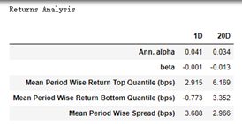
alpha是年化的超额收益,beta是市场暴露,这两个值是用市场均值和因子加权组合作为自变量和因变量做回归,残差就是alpha,回归系数就是beta。
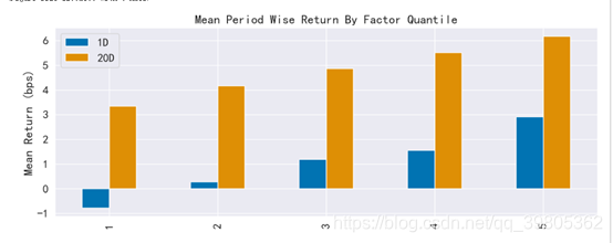
long_short是False时可以得到下面的图,long_short就是是否进行demean操作,false也就是说不尽兴demean操作,得到收益的绝对值。
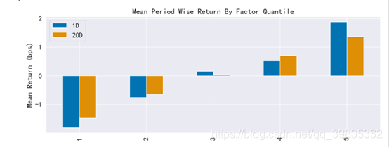
long_short是True时可以得到下面的图,long_short就是是否进行demean操作,True也就是说进行demean操作,得到收益的demean值,超出市场的收益情况。
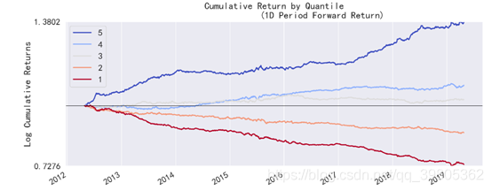

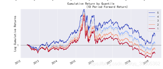
上图是Factor Weighted的图,也就是说这张图是用(因子值/所有因子值绝对值的和)的大小作为权重,去乘上对应的收益后加起来得到的,其余的mean的图都是直接取平均的,没有用因子值作为加权的。
如果说demean情况,也就是说参数long_short=True,那么会先对因子值做去中心化操作,然后用(因子值/所有因子值绝对值的和)的大小作为权重,去乘上对应的收益后加起来得到的。这也就是说做多因子大的,做空因子小的,然后和市场平均情况相比能得到的收益情况。
5、换手率分析
@plotting.customize
def create_turnover_tear_sheet(factor_data, turnover_periods=None):
    """
    Creates a tear sheet for analyzing the turnover properties of a factor.

    Parameters
    ----------
    factor_data : pd.DataFrame - MultiIndex
        A MultiIndex DataFrame indexed by date (level 0) and asset (level 1),
        containing the values for a single alpha factor, forward returns for
        each period, the factor quantile/bin that factor value belongs to, and
        (optionally) the group the asset belongs to.
        - See full explanation in utils.get_clean_factor_and_forward_returns
    turnover_periods : sequence[string], optional
        Periods to compute turnover analysis on. By default periods in
        'factor_data' are used but custom periods can provided instead. This
        can be useful when periods in 'factor_data' are not multiples of the
        frequency at which factor values are computed i.e. the periods
        are 2h and 4h and the factor is computed daily and so values like
        ['1D', '2D'] could be used instead
    """

    if turnover_periods is None:
        turnover_periods = utils.get_forward_returns_columns(
            factor_data.columns)

    quantile_factor = factor_data['factor_quantile']

    quantile_turnover = \
        {p: pd.concat([perf.quantile_turnover(quantile_factor, q, p)
                       for q in range(1, int(quantile_factor.max()) + 1)],
                      axis=1)
            for p in turnover_periods}

    autocorrelation = pd.concat(
        [perf.factor_rank_autocorrelation(factor_data, period) for period in
         turnover_periods], axis=1)

    plotting.plot_turnover_table(autocorrelation, quantile_turnover)

    fr_cols = len(turnover_periods)
    columns_wide = 1
    rows_when_wide = (((fr_cols - 1) // 1) + 1)
    vertical_sections = fr_cols + 3 * rows_when_wide + 2 * fr_cols
    gf = GridFigure(rows=vertical_sections, cols=columns_wide)

    for period in turnover_periods:
        if quantile_turnover[period].isnull().all().all():
            continue
        plotting.plot_top_bottom_quantile_turnover(quantile_turnover[period],
                                                   period=period,
                                                   ax=gf.next_row())

    for period in autocorrelation:
        if autocorrelation[period].isnull().all():
            continue
        plotting.plot_factor_rank_auto_correlation(autocorrelation[period],
                                                   period=period,
                                                   ax=gf.next_row())

    plt.show()
    gf.close()
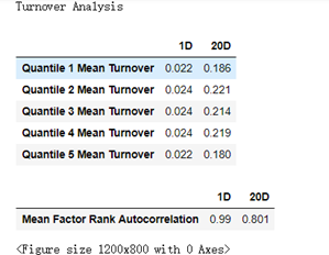
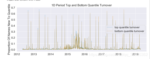
该函数生成2个,1、换手率表;2、换手率图
这里的换手率指的是该交易周期有的股票但是上一个交易周期没有的股票数量占该周期所有股票的数量。
6、事件分析
好啦!最后一个要说的函数了:create_event_study_tear_sheet,源码见下面吧,这个函数是用来研究一个特定事件,或分析各个周期的收益情况的。
@plotting.customize
def create_event_study_tear_sheet(factor_data,
                                  prices=None,
                                  avgretplot=(5, 15),
                                  rate_of_ret=True,
                                  n_bars=50):
    """
    Creates an event study tear sheet for analysis of a specific event.

    Parameters
    ----------
    factor_data : pd.DataFrame - MultiIndex
        A MultiIndex DataFrame indexed by date (level 0) and asset (level 1),
        containing the values for a single event, forward returns for each
        period, the factor quantile/bin that factor value belongs to, and
        (optionally) the group the asset belongs to.
    prices : pd.DataFrame, required only if 'avgretplot' is provided
        A DataFrame indexed by date with assets in the columns containing the
        pricing data.
        - See full explanation in utils.get_clean_factor_and_forward_returns
    avgretplot: tuple (int, int) - (before, after), optional
        If not None, plot event style average cumulative returns within a
        window (pre and post event).
    rate_of_ret : bool, optional
        Display rate of return instead of simple return in 'Mean Period Wise
        Return By Factor Quantile' and 'Period Wise Return By Factor Quantile'
        plots
    n_bars : int, optional
        Number of bars in event distribution plot
    """

    long_short = False

    plotting.plot_quantile_statistics_table(factor_data)

    gf = GridFigure(rows=1, cols=1)
    plotting.plot_events_distribution(events=factor_data['factor'],
                                      num_bars=n_bars,
                                      ax=gf.next_row())
    plt.show()
    gf.close()

    if prices is not None and avgretplot is not None:

        create_event_returns_tear_sheet(factor_data=factor_data,
                                        prices=prices,
                                        avgretplot=avgretplot,
                                        long_short=long_short,
                                        group_neutral=False,
                                        std_bar=True,
                                        by_group=False)

    factor_returns = perf.factor_returns(factor_data,
                                         demeaned=False,
                                         equal_weight=True)

    mean_quant_ret, std_quantile = \
        perf.mean_return_by_quantile(factor_data,
                                     by_group=False,
                                     demeaned=long_short)
    if rate_of_ret:
        mean_quant_ret = \
            mean_quant_ret.apply(utils.rate_of_return, axis=0,
                                 base_period=mean_quant_ret.columns[0])

    mean_quant_ret_bydate, std_quant_daily = \
        perf.mean_return_by_quantile(factor_data,
                                     by_date=True,
                                     by_group=False,
                                     demeaned=long_short)
    if rate_of_ret:
        mean_quant_ret_bydate = mean_quant_ret_bydate.apply(
            utils.rate_of_return, axis=0,
            base_period=mean_quant_ret_bydate.columns[0]
        )

    fr_cols = len(factor_returns.columns)
    vertical_sections = 2 + fr_cols * 1
    gf = GridFigure(rows=vertical_sections, cols=1)

    plotting.plot_quantile_returns_bar(mean_quant_ret,
                                       by_group=False,
                                       ylim_percentiles=None,
                                       ax=gf.next_row())

    plotting.plot_quantile_returns_violin(mean_quant_ret_bydate,
                                          ylim_percentiles=(1, 99),
                                          ax=gf.next_row())

    trading_calendar = factor_data.index.levels[0].freq
    if trading_calendar is None:
        trading_calendar = pd.tseries.offsets.BDay()
        warnings.warn(
            "'freq' not set in factor_data index: assuming business day",
            UserWarning
        )

    for p in factor_returns:

        plotting.plot_cumulative_returns(
            factor_returns[p],
            period=p,
            freq=trading_calendar,
            ax=gf.next_row()
        )

    plt.show()
    gf.close()
——————————————————————————————————————————————
最后的事件分析我也没有理解是啥意思,看了下源码暂且我的理解是每一天都作为中心然后向前向后分别计算累计收益,然后对各天求平均,得到中心向前向后的的各个分组的累计收益情况。但是搞不懂在实际中这个能说明啥东西,欢迎大佬在评论区指教,后续有新的理解也会再来补充。
