参考:
1、《Python机器学习:预测分析核心算法》 Michael Bowles P251-P258
 1 import numpy
 2
 3 #以前使用train_test_split构建训练和测试集, 但目前train_test_split已被cross_validation被废弃了
 4 #from sklearn.cross_validation import train_test_split
 5 #现在改为从 sklearn.model_selection 中调用train_test_split 函数可以解决此问题
 6 #感谢“简书 Junes_K” https://www.jianshu.com/p/d746c9e10b2f
 7 from sklearn.model_selection import train_test_split
 8
 9 #可以构建sklearn.ensemble.RandomForestRegressor对象
10 from sklearn import ensemble
11
12 #用mean_squared_error来计算预测均方误差
13 from sklearn.metrics import mean_squared_error
14
15 import pylab as plot
16
17 # 从本机读取数据
18 target_file = open('winequality-red.csv','r')
19 data = target_file.readlines()
20 target_file.close()
21
22 #整理原始数据,将原始数据分为属性列表(xList),标签列表(labels)
23 #将各个属性的名称存入names列表
24 xList = []
25 labels = []
26 names = []
27 firstLine = True
28 for line in data:
29     if firstLine:
30         names = line.strip().split(";")
31         firstLine = False
32     else:
33         #split on semi-colon
34         row = line.strip().split(";")
35         #put labels in separate array
36         labels.append(float(row[-1]))
37         #remove label from row
38         row.pop()
39         #convert row to floats
40         floatRow = [float(num) for num in row]
41         xList.append(floatRow)
42
43 #计算属性列表的行数和列数
44 nrows = len(xList)
45 ncols = len(xList[0])
46
47 #将各列表转为numpy数组形式,此形式是RandomForestRegressor的要求
48 #并且这些对象可以使用sklearn的train_test_split构建训练和测试集
49 X = numpy.array(xList)
50 y = numpy.array(labels)
51 wineNames = numpy.array(names)
52
53 #构建test集为30%规模的训练集和测试集
54 #random_state设置为一个特殊整数,而不是让随机数生成器自己选择一个不可重复的内部值
55 #这样重复代码可以获得同样的结果,便于开发阶段的调整,否则随机性会掩盖所做的改变
56 #固定random_state就固定了测试集,会对测试数据集过度训练
57 xTrain, xTest, yTrain, yTest = train_test_split(X, y, test_size=0.30, random_state=531)
58
59 #train random forest at a range of ensemble sizes in order to see how the mse changes
60 mseOos = []
61 nTreeList = range(50, 500, 10)
62 for iTrees in nTreeList:
63     depth = None
64     maxFeat  = 4
65     #https://scikit-learn.org/stable/modules/generated/sklearn.ensemble.RandomForestRegressor.html#sklearn.ensemble.RandomForestRegressor
66     #初始化RandomForestRegressor对象
67     #通过n_estimators = iTrees(属于nTreeList)来确定决策树的数目,这里是从50到500,每隔10的整数
68     #max_depth = depth为None,决策树会持续增长,直到叶子节点为空或者所含数据小于min_sample_split
69     #这里min_sample_split使用了缺省值(为2),当节点含有的数据小于其时,此节点不再分割
70     #max_features = maxFeat,从而保证每次随机考虑四个属性,而不是要考虑全部属性,否则就是Bagging方法了
71     #oob_score = False,不使用袋外样本估算看不见的数据的(有的不明白),缺省值为False
72     wineRFModel = ensemble.RandomForestRegressor(n_estimators=iTrees, max_depth=depth, max_features=maxFeat,random_state=531)
73
74     #调用fit()方法,训练数据集作为输入参数
75     wineRFModel.fit(xTrain,yTrain)
76
77     #调用predict()进行预测,输入时测试集的数据
78     prediction = wineRFModel.predict(xTest)
79     #将预测值与测试集中的标签比较,用mean_squared_error来计算预测均方误差
80     mseOos.append(mean_squared_error(yTest, prediction))
81
82 #打印最后一个均方误差,这里并不代表最小值
83 #随机森林产生近乎独立的预测,然后取它们的平均值。因为为平均值,增加更多的决策树不会导致过度拟合。
84 print("MSE" )
85 print(mseOos[-1])
程序运行后得到:
MSE
0.318127065111759
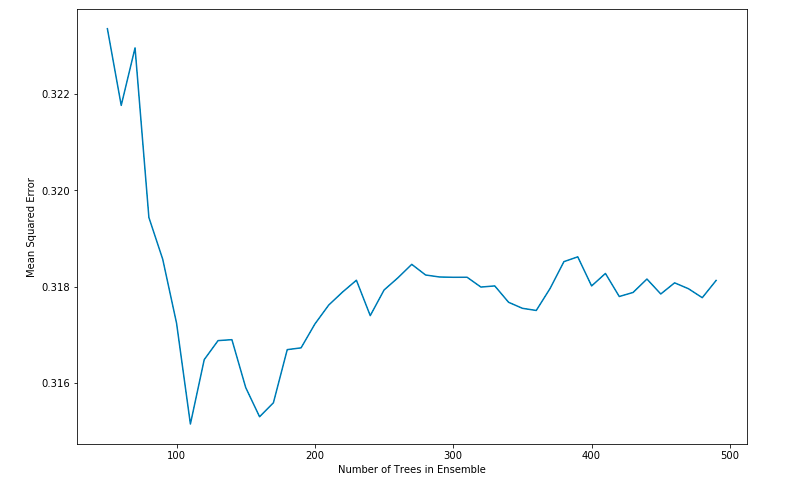
 1 #plot training and test errors vs number of trees in ensemble
 2 plot.figure(figsize=(12,8))
 3 plot.plot(nTreeList, mseOos)
 4 plot.xlabel('Number of Trees in Ensemble')
 5 plot.ylabel('Mean Squared Error')
 6 plot.show()
 7
 8 #从下图也可以看出最后一个均方差并不是最小值,最小值是统计上的波动造成的,不是可以重复的最小值。
 9 #同时曲线展示了随机森林算法的减少方差的特性
10 #原书上的:随着决策树数目增加,预测误差在下降,曲线波动也在减小(本例中不是太明显)
程序运行后得到:
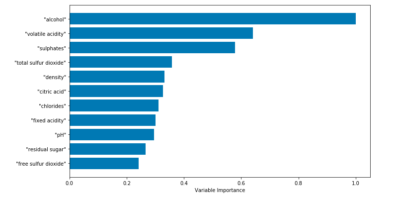
 1 # feature_importances是一个数组,数组长度等于属性的个数
 2 #数组中的值为正的浮点数,表面对应属性对预测结果的重要性
 3 featureImportance = wineRFModel.feature_importances_
 4
 5 #对属性重要性归一化,按照属性重要程度排序
 6 featureImportance = featureImportance / featureImportance.max()
 7
 8 sorted_idx = numpy.argsort(featureImportance)
 9 barPos = numpy.arange(sorted_idx.shape[0]) + .5
10 plot.figure(figsize=(12,6))
11 plot.barh(barPos, featureImportance[sorted_idx], align='center')
12 plot.yticks(barPos, wineNames[sorted_idx])
13 plot.xlabel('Variable Importance')
14 plot.subplots_adjust(left=0.2, right=0.9, top=0.9, bottom=0.1)
15 plot.show()
程序运行后得到: