1处理文本数据

文本是一种以字符或者单词为序列数据，而如何让他让计算机读懂从而进行一系列处理是比较关键的一步。从本质上来说文字其实就是便于人这种碳基生命理解的抽象符号，而对于计算机这种硅基生命胚胎来说，或许向量才是它们最便于理解的形式，因此下面介绍如何将文本向量化。
将文本分解成的单元叫做标记，将文本分解成标记的过程叫做分词。标记有单词、字符和单词或字符的n-grame三种，其中n-grame很少用于深度学习，这里不再多说。而向量和标记相关联的方法主要有两种，一种为one-hot编码，一种为标记嵌入（包含词嵌入(word embedding)）

单词和字符的one-hot编码

单词级的one-hot编码

import numpy as np

samples = ['The cat sat on the mat.', 'The dog ate my homework.']
token_index = {}
for sample in samples:
    for word in sample.split():
        if word not in token_index:
            token_index[word] = len(token_index) + 1
max_length = 10
results = np.zeros((len(samples), max_length, max(token_index.values()) + 1))
for i, sample in enumerate(samples):
    for j, word in list(enumerate(sample.split()))[:max_length]:
        index = token_index.get(word)
        results[i, j, index] = 1.

调用keras API实现单词级分类

from keras.preprocessing.text import Tokenizer

samples = ['The cat sat on the mat.', 'The dog ate my homework.']
#创建一个分词器（tokenizer）只考虑前1000个常见单词
tokenizer = Tokenizer(num_words=1000)
构建单词索引
tokenizer.fit_on_texts(samples)

将字符串转化成为整数索引组成的列表
sequences = tokenizer.texts_to_sequences(samples)

得到one-hot编码的二进制表示
one_hot_results = tokenizer.texts_to_matrix(samples, mode='binary')

找回单词引索
word_index = tokenizer.word_index
print('Found %s unique tokens.' % len(word_index))

使用词嵌入

有没有一个理想的词嵌入空间，可以完美映射人类语言，并可用于所有自然语言处理任务？可能有，但我们尚未发现。因此合理的做法是对每个新任务都学习一个新的嵌入空间。

利用Embedding层学习词嵌入

IMDB数据集是Keras内部集成的，初次导入需要下载一下，之后就可以直接用了。
IMDB数据集包含来自互联网的50000条严重两极分化的评论，该数据被分为用于训练的25000条评论和用于测试的25000条评论，训练集和测试集都包含50%的正面评价和50%的负面评价。该数据集已经经过预处理：评论（单词序列）已经被转换为整数序列，其中每个整数代表字典中的某个单词。

from keras.layers import Embedding
from keras.datasets import imdb
from keras import preprocessing
from keras.models import Sequential
from keras.layers import Flatten, Dense
embedding_layer = Embedding(1000, 64)


# Number of words to consider as features
max_features = 10000
# Cut texts after this number of words
# (among top max_features most common words)
maxlen = 20

# Load the data as lists of integers.
(x_train, y_train), (x_test, y_test) = imdb.load_data(num_words=max_features)


#查看内容
word_index = imdb.get_word_index()
reverse_word_index = dict([(value, key) for (key, value) in word_index.items()])
decoded_review = ' '.join([reverse_word_index.get(i - 3, '?') for i in x_train[0]])
print(decoded_review)

x_train = preprocessing.sequence.pad_sequences(x_train, maxlen=maxlen)
x_test = preprocessing.sequence.pad_sequences(x_test, maxlen=maxlen)



model = Sequential()
model.add(Embedding(10000, 8, input_length=maxlen))
model.add(Flatten())
model.add(Dense(1, activation='sigmoid'))
model.compile(optimizer='rmsprop', loss='binary_crossentropy', metrics=['acc'])
model.summary()

history = model.fit(x_train, y_train,
                    epochs=10,
                    batch_size=32,
                    validation_split=0.2)

结果
在这里插入图片描述

从原始文本到词嵌入

原始文本读取与标签制作

这里选择IMDB原始数据集，不同与上一节keras内置的数据集，我们这次要自己进行分词和数字映射，并根据评论标签给数据集制作labels列表。

import os
#你自己的数据集路径
imdb_dir = 'aclImdb'
train_dir = os.path.join(imdb_dir, 'train')

labels = []
texts = []

for label_type in ['neg', 'pos']:
    dir_name = os.path.join(train_dir, label_type)
    for fname in os.listdir(dir_name):
        if fname[-4:] == '.txt':
            f = open(os.path.join(dir_name, fname),errors="ignore")#注意errors="ignore"一定要加，要不报错
            texts.append(f.read())
            f.close()
            if label_type == 'neg':
                labels.append(0)
            else:
                labels.append(1)

对数据进行分词

这里使用分词器tokenizer，常见的使用方式见这里,下面对文本进行分词，并划分训练集和测试集。

maxlen = 100  # We will cut reviews after 100 words
training_samples = 200  # We will be training on 200 samples
validation_samples = 10000  # We will be validating on 10000 samples
max_words = 10000  # We will only consider the top 10,000 words in the dataset

tokenizer = Tokenizer(num_words=max_words)
tokenizer.fit_on_texts(texts)
sequences = tokenizer.texts_to_sequences(texts)
print(len(sequences))
word_index = tokenizer.word_index
print('Found %s unique tokens.' % len(word_index))
#把序列补成一样的长度
data = pad_sequences(sequences, maxlen=maxlen)

labels = np.asarray(labels)
print('Shape of data tensor:', data.shape)
print('Shape of label tensor:', labels.shape)


indices = np.arange(data.shape[0])
#打乱顺序
np.random.shuffle(indices)
data = data[indices]
labels = labels[indices]

x_train = data[:training_samples]
y_train = labels[:training_samples]
x_val = data[training_samples: training_samples + validation_samples]
y_val = labels[training_samples: training_samples + validation_samples]

使用CloVe进行词嵌入

从这里下载2014年英文维基百科的预计算嵌入。文件名为glove.6B.zip,包含400000个单词。然后我们使用其中的一个文件构建一个将单词映射为其向量表示的引索，得到一个embeddings_index字典，{单词:单词向量}

扫描二维码关注公众号，回复： 9115098 查看本文章

glove_dir = ''

embeddings_index = {}
f = open(os.path.join(glove_dir, 'glove.6B.300d.txt'),errors="ignore")
for line in f:
    values = line.split()
    word = values[0]
    coefs = np.asarray(values[1:], dtype='float32')
    embeddings_index[word] = coefs
f.close()

print('Found %s word vectors.' % len(embeddings_index))

然后准备GloVe词嵌入矩阵

embedding_dim = 300

embedding_matrix = np.zeros((max_words, embedding_dim))
for word, i in word_index.items():
    embedding_vector = embeddings_index.get(word)
    if i < max_words:
        if embedding_vector is not None:
            # Words not found in embedding index will be all-zeros.
            embedding_matrix[i] = embedding_vector

然后定义模型

from keras.models import Sequential
from keras.layers import Embedding, Flatten, Dense

model = Sequential()
model.add(Embedding(max_words, embedding_dim, input_length=maxlen))
model.add(Flatten())
model.add(Dense(32, activation='relu'))
model.add(Dense(1, activation='sigmoid'))
model.summary()

在模型中中添加GloVe嵌入,并进行微调训练及可视化

model.layers[0].set_weights([embedding_matrix])
model.layers[0].trainable = False

model.compile(optimizer='rmsprop',
              loss='binary_crossentropy',
              metrics=['acc'])
history = model.fit(x_train, y_train,
                    epochs=10,
                    batch_size=32,
                    validation_data=(x_val, y_val))
model.save_weights('pre_trained_glove_model.h5')

import matplotlib.pyplot as plt

acc = history.history['acc']
val_acc = history.history['val_acc']
loss = history.history['loss']
val_loss = history.history['val_loss']

epochs = range(1, len(acc) + 1)

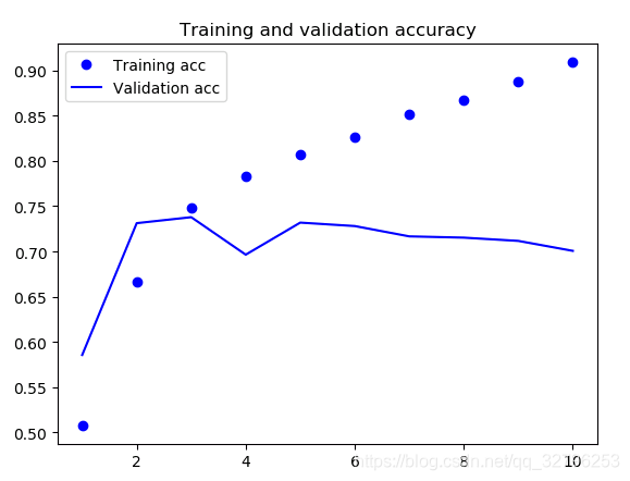
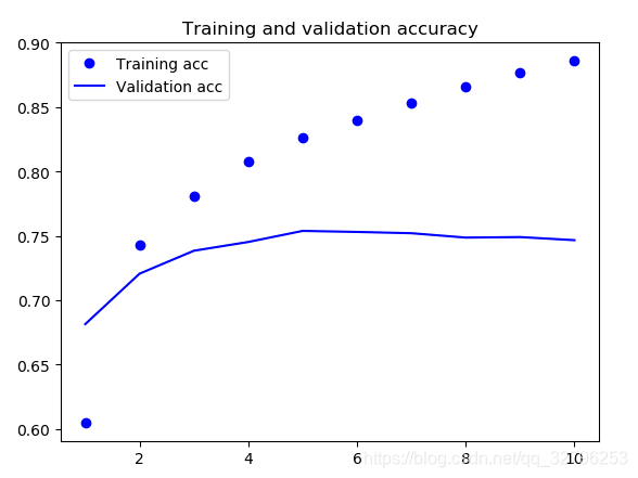
plt.plot(epochs, acc, 'bo', label='Training acc')
plt.plot(epochs, val_acc, 'b', label='Validation acc')
plt.title('Training and validation accuracy')
plt.legend()

plt.figure()

plt.plot(epochs, loss, 'bo', label='Training loss')
plt.plot(epochs, val_loss, 'b', label='Validation loss')
plt.title('Training and validation loss')
plt.legend()

plt.show()