《动手学》Pytorch版课程笔记——第一期

概述

在疫情期间宅在家中，偶然得到伯禹教育公益课程，整个课程体系非常系统地介绍了深度学习的体系，但最吸引我的还是pytorch的教学和使用，因为之前因为torch不太会，在看nlp竞赛开源方案时有点麻烦。一次开了一个小小的专题，记录一下为期14天的课程，系统巩固一下知识。整个课程的参考书籍为《动手学深度学习》
第一期笔记主要是前三讲线性回归、softmax和多层感知器，主要从非库函数版和库函数版两个角度来分别呈现算法的原理和工程实践。

1.线性回归

针对这方面知识，举个简单例子，这里我们假设价格只取决于房屋状况的两个因素，即面积（平方米）和房龄（年）。接下来我们希望探索价格与这两个因素的具体关系。线性回归假设输出与各个输入之间是线性关系:
$\mathrm{price} = w_{\mathrm{area}} \cdot \mathrm{area} + w_{\mathrm{age}} \cdot \mathrm{age} + b$
然后就是损失函数和优化方式，这里分别列出数据生成、网络搭建，损失函数与SGD的非库函数版实现：

• 数据随机生成
  这里介绍如何随机生成可验证模型的随机数据，方便测自己搭建模型是否有效。

# set input feature number 
num_inputs = 2
# set example number
num_examples = 1000

# set true weight and bias in order to generate corresponded label
true_w = [2, -3.4]
true_b = 4.2

features = torch.randn(num_examples, num_inputs,
                      dtype=torch.float32)
labels = true_w[0] * features[:, 0] + true_w[1] * features[:, 1] + true_b
labels += torch.tensor(np.random.normal(0, 0.01, size=labels.size()),
                       dtype=torch.float32)

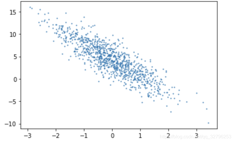
可视化一下随机生成数据

plt.scatter(features[:, 1].numpy(), labels.numpy(), 1);

生成完数据就是加载数据环节了，为了增加读取效率和节约空间，这里用生成器来读取

def data_iter(batch_size, features, labels):
    num_examples = len(features)
    indices = list(range(num_examples))
    random.shuffle(indices)  # random read 10 samples
    for i in range(0, num_examples, batch_size):
        j = torch.LongTensor(indices[i: min(i + batch_size, num_examples)]) # the last time may be not enough for a whole batch
        yield  features.index_select(0, j), labels.index_select(0, j)

• 定义模型版
  1 损失函数
  $l^{(i)}(\mathbf{w}, b) = \frac{1}{2} \left(\hat{y}^{(i)} - y^{(i)}\right)^2,$
  2 优化函数
  $(\mathbf{w},b) \leftarrow (\mathbf{w},b) - \frac{\eta}{|\mathcal{B}|} \sum_{i \in \mathcal{B}} \partial_{(\mathbf{w},b)} l^{(i)}(\mathbf{w},b)$

# 参数初始化
w = torch.tensor(np.random.normal(0, 0.01, (num_inputs, 1)), dtype=torch.float32)
b = torch.zeros(1, dtype=torch.float32)
w.requires_grad_(requires_grad=True)
b.requires_grad_(requires_grad=True)
# 定义网络结构
def linreg(X, w, b):
    return torch.mm(X, w) + b
# 定义损失函数
def squared_loss(y_hat, y): 
    return (y_hat - y.view(y_hat.size())) ** 2 / 2
# 定义优化函数
def sgd(params, lr, batch_size): 
    for param in params:
        param.data -= lr * param.grad / batch_size # ues .data to operate param without gradient track

# 模型训练
# super parameters init
lr = 0.03
num_epochs = 5

net = linreg
loss = squared_loss

# training
for epoch in range(num_epochs):  # training repeats num_epochs times
    # in each epoch, all the samples in dataset will be used once
    
    # X is the feature and y is the label of a batch sample
    for X, y in data_iter(batch_size, features, labels):
        l = loss(net(X, w, b), y).sum()  
        # calculate the gradient of batch sample loss 
        l.backward()  
        # using small batch random gradient descent to iter model parameters
        sgd([w, b], lr, batch_size)  
        # reset parameter gradient
        w.grad.data.zero_()
        b.grad.data.zero_()
    train_l = loss(net(features, w, b), labels)
    print('epoch %d, loss %f' % (epoch + 1, train_l.mean().item()))

• 简洁版

import torch
from torch import nn
import numpy as np
torch.manual_seed(1)

print(torch.__version__)
torch.set_default_tensor_type('torch.FloatTensor')


num_inputs = 2
num_examples = 1000

true_w = [2, -3.4]
true_b = 4.2

features = torch.tensor(np.random.normal(0, 1, (num_examples, num_inputs)), dtype=torch.float)
labels = true_w[0] * features[:, 0] + true_w[1] * features[:, 1] + true_b
labels += torch.tensor(np.random.normal(0, 0.01, size=labels.size()), dtype=torch.float)

import torch.utils.data as Data

batch_size = 10

# combine featues and labels of dataset
dataset = Data.TensorDataset(features, labels)

# put dataset into DataLoader
data_iter = Data.DataLoader(
    dataset=dataset,            # torch TensorDataset format
    batch_size=batch_size,      # mini batch size
    shuffle=True,               # whether shuffle the data or not
    num_workers=2,              # read data in multithreading
)

以下是三种简历模型的方式

# ways to init a multilayer network
# method one
net = nn.Sequential(
    nn.Linear(num_inputs, 1)
    # other layers can be added here
    )

# method two
net = nn.Sequential()
net.add_module('linear', nn.Linear(num_inputs, 1))
# net.add_module ......

# method three
from collections import OrderedDict
net = nn.Sequential(OrderedDict([
          ('linear', nn.Linear(num_inputs, 1))
          # ......
        ]))

#模型初始化如下：
from torch.nn import init

init.normal_(net[0].weight, mean=0.0, std=0.01)
init.constant_(net[0].bias, val=0.0)  # or you can use net[0].bias.data.fill_(0)` to modify it directly
#定义损失函数
loss = nn.MSELoss()    # nn built-in squared loss function
                       # function prototype: `torch.nn.MSELoss(size_average=None, reduce=None, reduction='mean')
#定义优化函数
import torch.optim as optim

optimizer = optim.SGD(net.parameters(), lr=0.03)   # built-in random gradient descent function
 # function prototype: `torch.optim.SGD(params, lr=, momentum=0, dampening=0, weight_decay=0, nesterov=False)
# 训练网络
num_epochs = 3
for epoch in range(1, num_epochs + 1):
    for X, y in data_iter:
        output = net(X)
        l = loss(output, y.view(-1, 1))
        optimizer.zero_grad() # reset gradient, equal to net.zero_grad()
        l.backward()
        optimizer.step()
    print('epoch %d, loss: %f' % (epoch, l.item()))

详解torch中的backward()函数，以及pytorch的2种求导方法

2 softmax

本节课主要讲解了如何用线性模型做一个分类，本博文主要在此记录一下torch的一些轮子，以及torchvision的一些轮子；
这里我们会使用torchvision包，它是服务于PyTorch深度学习框架的，主要用来构建计算机视觉模型。torchvision主要由以下几部分构成：

1. torchvision.datasets: 一些加载数据的函数及常用的数据集接口；
2. torchvision.models: 包含常用的模型结构（含预训练模型），例如AlexNet、VGG、ResNet等；
3. torchvision.transforms: 常用的图片变换，例如裁剪、旋转等；
4. torchvision.utils: 其他的一些有用的方法。

softmax的公式：
$\hat{y}_j = \frac{ \exp(o_j)}{\sum_{i=1}^3 \exp(o_i)} \\ \ \\ \begin{aligned} \boldsymbol{o}^{(i)} &= \boldsymbol{x}^{(i)} \boldsymbol{W} + \boldsymbol{b},\\ \boldsymbol{\hat{y}}^{(i)} &= \text{softmax}(\boldsymbol{o}^{(i)}). \end{aligned}$

def softmax(X):
    X_exp = X.exp()
    partition = X_exp.sum(dim=1, keepdim=True)
    # print("X size is ", X_exp.size())
    # print("partition size is ", partition, partition.size())
    return X_exp / partition  # 这里应用了广播机制

def net(X):
    return softmax(torch.mm(X.view((-1, num_inputs)), W) + b)
# 损失函数
def cross_entropy(y_hat, y):
    return - torch.log(y_hat.gather(1, y.view(-1, 1)))
# 准确率
def accuracy(y_hat, y):
    return (y_hat.argmax(dim=1) == y).float().mean().item()

几个小知识点：

• torch.mm是指矩阵相乘，torch.mul是矩阵点乘，x.view相当于reshape

• gather的api:
  torch.gather(input, dim, index, out=None) → Tensor
  dim轴，index的形状是输出的形状一致。

• x.item()得到张量的元素值

3多层感知器

3.1 激活函数
如果将隐藏层的输出直接作为输出层的输入可以得到
$\boldsymbol{O} = (\boldsymbol{X} \boldsymbol{W}_h + \boldsymbol{b}_h)\boldsymbol{W}_o + \boldsymbol{b}_o = \boldsymbol{X} \boldsymbol{W}_h\boldsymbol{W}_o + \boldsymbol{b}_h \boldsymbol{W}_o + \boldsymbol{b}_o.$
从上面的式子可以看出，虽然神经网络引入了隐藏层，却依然等价于一个单层神经网络：其中输出层权重参数为 $\boldsymbol{W}_h\boldsymbol{W}_o$，偏差参数为 $\boldsymbol{b}_h \boldsymbol{W}_o + \boldsymbol{b}_o$。不难发现，即便再添加更多的隐藏层，以上设计依然只能与仅含输出层的单层神经网络等价。

上述问题的根源在于全连接层只是对数据做仿射变换（affine transformation），而多个仿射变换的叠加仍然是一个仿射变换。解决问题的一个方法是引入非线性变换，例如对隐藏变量使用按元素运算的非线性函数进行变换，然后再作为下一个全连接层的输入。这个非线性函数被称为激活函数（activation function）。

这里重点记录一下激活函数的求导和选择，关于为什么要y.sum().backward()还是有点一知半解，希望以后能更加清晰。

• 求导

x = torch.arange(-8.0, 8.0, 0.1, requires_grad=True)
y = x.relu()
xyplot(x, y, 'relu')
y.sum().backward()

• 选择
  ReLu函数是一个通用的激活函数，目前在大多数情况下使用。但是，ReLU函数只能在隐藏层中使用。用于分类器时，sigmoid函数及其组合通常效果更好。由于梯度消失问题，有时要避免使用sigmoid和tanh函数。 在神经网络层数较多的时候，最好使用ReLu函数，ReLu函数比较简单计算量少，而sigmoid和tanh函数计算量大很多。在选择激活函数的时候可以先选用ReLu函数如果效果不理想可以尝试其他激活函数。

3.2 从头搭建

num_inputs, num_outputs, num_hiddens = 784, 10, 256

W1 = torch.tensor(np.random.normal(0, 0.01, (num_inputs, num_hiddens)), dtype=torch.float)
b1 = torch.zeros(num_hiddens, dtype=torch.float)
W2 = torch.tensor(np.random.normal(0, 0.01, (num_hiddens, num_outputs)), dtype=torch.float)
b2 = torch.zeros(num_outputs, dtype=torch.float)
params = [W1, b1, W2, b2]

for param in params:
    param.requires_grad_(requires_grad=True)

def relu(X):
    return torch.max(input=X, other=torch.tensor(0.0))
def net(X):
    X = X.view((-1, num_inputs))
    H = relu(torch.matmul(X, W1) + b1)
    return torch.matmul(H, W2) + b2