揭开深度强化学习的神秘面纱

参考资料

• https://neuro.cs.ut.ee/demystifying-deep-reinforcement-learning/

---

强化学习

---

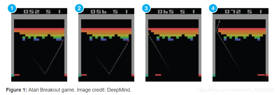
考虑游戏Breakout。 在这个游戏中你可以控制屏幕底部的一个球拍，并且必须将球弹回以清除屏幕上半部分的所有砖块。 每当你打砖，它就会消失，你的分数会增加 - 你会获得奖励。

Consider the game Breakout. In this game you control a paddle at the bottom of the screen and have to bounce the ball back to clear all the bricks in the upper half of the screen. Each time you hit a brick, it disappears and your score increases – you get a reward.

假设您想教一个神经网络来玩这个游戏。 您的网络输入将是屏幕图像，输出将是三个动作：左，右或火（发射球）。 将它视为一个分类问题是有意义的 - 对于你必须决定的每个游戏屏幕，你是应该左右移动还是按火。 听起来很简单？ 当然，但是你需要训练样例和很多例子。 当然，您可以使用专业玩家去录制游戏会话，但这并不是我们学习的方式。 我们不需要有人告诉我们一百万次在每个屏幕上选择哪一个。 我们只是需要偶尔的反馈，我们做了正确的事情，然后我们可以自己弄清楚其他一切。

Suppose you want to teach a neural network to play this game. Input to your network would be screen images, and output would be three actions: left, right or fire (to launch the ball). It would make sense to treat it as a classification problem – for each game screen you have to decide, whether you should move left, right or press fire. Sounds straightforward? Sure, but then you need training examples, and a lots of them. Of course you could go and record game sessions using expert players, but that’s not really how we learn. We don’t need somebody to tell us a million times which move to choose at each screen. We just need occasional feedback that we did the right thing and can then figure out everything else ourselves.

这是任务强化学习试图解决的问题。 强化学习介于有监督和无监督学习之间。 在有监督的学习中，每个训练样本都有一个目标标签，而在无监督学习中，一个人根本没有标签，在强化学习中，一个人有稀疏和延时的标签 - 奖励。 仅基于这些奖励，agent必须学会在环境中行事。

This is the task reinforcement learning tries to solve. Reinforcement learning lies somewhere in between supervised and unsupervised learning. Whereas in supervised learning one has a target label for each training example and in unsupervised learning one has no labels at all, in reinforcement learning one has sparse and time-delayed labels – the rewards. Based only on those rewards the agent has to learn to behave in the environment.

虽然这个想法非常直观，但在实践中存在许多挑战。 例如，当你在Breakout游戏中打砖并获得奖励时，它通常与你在获得奖励之前所做的动作（划桨动作）无关。 当你正确定位球拍并将球弹回来时，所有的努力工作都已经完成。 这被称为信用分配问题 - 即，前面的哪些行为负责获得奖励以及在何种程度上。

While the idea is quite intuitive, in practice there are numerous challenges. For example when you hit a brick and score a reward in the Breakout game, it often has nothing to do with the actions (paddle movements) you did just before getting the reward. All the hard work was already done, when you positioned the paddle correctly and bounced the ball back. This is called the credit assignment problem – i.e., which of the preceding actions were responsible for getting the reward and to what extent.

一旦你想出了收集一定数量奖励的策略，你应该坚持下去或尝试一些可能带来更大奖励的东西吗？ 在上面的 Breakout 游戏中，一个简单的策略是移动到左边缘并在那里等待。 在发射时，球往往比右侧飞得更频繁，在你死之前你很容易在大约10分上得分。 你会对此感到满意还是想要更多？ 这被称为探索 - 利用困境 - 如果您利用已知的工作策略或探索其他可能更好的策略。

Once you have figured out a strategy to collect a certain number of rewards, should you stick with it or experiment with something that could result in even bigger rewards? In the above Breakout game a simple strategy is to move to the left edge and wait there. When launched, the ball tends to fly left more often than right and you will easily score on about 10 points before you die. Will you be satisfied with this or do you want more? This is called the explore-exploit dilemma – should you exploit the known working strategy or explore other, possibly better strategies.

强化学习是我们（以及所有动物）学习方式的重要模型。 来自父母的赞美，在校的成绩，工作中的薪水 - 这些都是奖励的例子。 商业和人际关系中每天都会出现信用分配问题和探索剥削困境。 这就是研究这个问题很重要的原因，游戏形成了一个用于尝试新方法的精彩沙箱。

Reinforcement learning is an important model of how we (and all animals in general) learn. Praise from our parents, grades in school, salary at work – these are all examples of rewards. Credit assignment problems and exploration-exploitation dilemmas come up every day both in business and in relationships. That’s why it is important to study this problem, and games form a wonderful sandbox for trying out new approaches.

---

马尔可夫决策过程

---

形式化一个强化学习问题的最常用方法是将其表示为马尔可夫决策过程。

假设您是一个位于环境中的agent(例如Breakout游戏)。环境处于一定的状态(如桨的位置、球的位置和方向、每块砖的存在等)。agent可以在环境中执行某些action(例如将桨向左或向右移动)。这些行为有时会带来回报(例如分数的增加)。action转换环境并导致一个新的状态，在这个状态中agent可以执行另一个action，等等。选择这些action的规则称为策略。一般来说，环境是随机的，这意味着下一个状态可能是随机的(例如，当你丢了一个球，然后发射了一个新的，它向着随机的方向)。

Suppose you are an agent, situated in an environment (e.g. Breakout game). The environment is in a certain state (e.g. location of the paddle, location and direction of the ball, existence of every brick and so on). The agent can perform certain actions in the environment (e.g. move the paddle to the left or to the right). These actions sometimes result in a reward (e.g. increase in score). Actions transform the environment and lead to a new state, where the agent can perform another action, and so on. The rules for how you choose those actions are called policy. The environment in general is stochastic, which means the next state may be somewhat random (e.g. when you lose a ball and launch a new one, it goes towards a random direction).

一组状态和行为，以及从一个状态转换到另一个状态和获得奖励的规则，构成了一个马尔可夫决策过程。这个过程中的一段 episode(例如一款游戏)形成了有限的状态、动作和奖励序列:
$s_0,a_0,r_1,s_1,a_1,r_2,s_2,…,s_{n−1},a_{n−1},r_n,s_n$

The set of states and actions, together with rules for transitioning from one state to another and for getting rewards, make up a Markov decision process. One episode of this process (e.g. one game) forms a finite sequence of states, actions and rewards:

---

折扣未来奖励

---

要想长期表现良好，我们不仅要考虑眼前的回报，还要考虑未来的回报。我们该怎么做呢?

To perform well in long-term, we need to take into account not only the immediate rewards, but also the future awards we are going to get. How should we go about that?

给定一个运行的马尔可夫决策过程，我们可以很容易地计算出一个episode的总回报:
$R=r_1+r_2+r_3+…+r_n$

Given one run of Markov decision process, we can easily calculate the total reward for one episode:

但由于我们的环境是随机的，我们永远无法确定，下次我们做同样的事情时，是否会得到同样的回报。我们越走向未来，分歧就越大。基于这个原因，我们通常会用折扣的未来奖励来代替:

$R_t=r_t+γr_{t+1}+γ^2r_{t+2}…+γ^{n−t}r_n$
$R_t=r_t+γ(r_{t+1}+γ(r_{t+2}+…))=r_t+γR_{t+1}$

这里 $\gamma$是折扣因子

But because our environment is stochastic, we can never be sure, if we will get the same rewards the next time we perform the same actions. The more into the future we go, the more it may diverge. For that reason it is common to use discounted future reward instead:

对于一个agent来说，一个好的策略是总是选择一个行为，以使未来的折扣回报最大化。

A good strategy for an agent would be to always choose an action, that maximizes the discounted future reward.

---

Q-learning

---

在Q-learning中，我们定义一个函数 $Q(s,a)$为:
$Q(s_t,a_t)=max_πR_{t+1}$
把 $Q(s,a)$看成:
这听起来可能是一个令人困惑的定义。如果我们只知道当前的状态和action，而不知道之后的action和奖励，我们怎么能在游戏结束时估计分数呢？我们真的做不到。但作为一个理论结构，我们可以假设存在这样一个函数。闭上眼睛，对自己重复五遍:Q(s,a)存在，Q(s,a)存在…，感觉到了吗？

This may sound quite a puzzling definition. How can we estimate the score at the end of game, if we know just current state and action, and not the actions and rewards coming after that? We really can’t. But as a theoretical construct we can assume existence of such a function. Just close your eyes and repeat to yourself five times: “Q(s,a) exists, Q(s,a) exists, …”. Feel it?

如果您仍然不相信，那么考虑一下拥有这样一个函数的含义。假设你处于s状态，正在考虑应该采取行动a还是行动b。 您想要选择一个动作，从而在游戏结束时获得最高分。 一旦你拥有神奇的Q函数，答案就变得非常简单 - 选择具有最高Q值的动作！

If you’re still not convinced, then consider what the implications of having such a function would be. Suppose you are in state s and pondering whether you should take action a or b. You want to select the action, that results in the highest score at the end of game. Once you have the magical Q-function, the answer becomes really simple – pick the action with the highest Q-value!

$π(s)=argmax_aQ(s,a)$

这里π代表策略，我们如何选择每个state的action。

那么我们怎么得到Q-function呢？我们只关注一个transition $<s,a,r,s'>$,就像上一节中折扣的未来奖励一样，我们可以用下一个状态 $s'$的Q值表示状态s和动作a的Q值。

$Q(s,a)=r+γmax_{a'}Q(s',a')$

这个方程叫做 Bellman 方程。如果你仔细想想，这是很合乎逻辑的——这种状态和行为的最大未来回报是即时回报加上下一种状态的最大未来回报。

Q-learning的主要思想是利用贝尔曼方程迭代逼近Q函数。在最简单的情况下，Q函数实现为表，状态为行，操作为列。Q-learning算法的要点简单如下:

initialize Q[numstates,numactions] arbitrarily
observe initial state s
repeat
  select and carry out an action a
  observe reward r and new state s’
  $Q[s,a] = Q[s,a] + α(r + γmax_{a'} Q[s',a'] - Q[s,a])$
  $s = s'$
until terminated

算法中的 $α$是学习率，其控制考虑先前Q值与新的Q值之间的差异的多少。

α in the algorithm is a learning rate that controls how much of the difference between previous Q-value and newly proposed Q-value is taken into account. In particular, when α=1, then two Q[s,a]-s cancel and the update is exactly the same as Bellman equation.

我们用来更新 $Q [s,a]$的 $max_{a'}Q [s',a']$只是一种估计，在学习的早期阶段，它可能是完全错误的。 然而，每次迭代的估计越来越准确，并且已经证明，如果我们执行此更新足够多次，那么Q函数将收敛并表示真实的Q值。

maxa’ Q[s’,a’] that we use to update Q[s,a] is only an estimation and in early stages of learning it may be completely wrong. However the estimations get more and more accurate with every iteration and it has been shown, that if we perform this update enough times, then the Q-function will converge and represent the true Q-value.

---

Deep Q Network

---

Breakout game中的环境状态可以通过球拍的位置，球的位置和方向以及每个单独砖的存在来定义。 然而，这种直观表示是游戏特定的。 我们能否提出更适合所有游戏的更普遍的东西？ 显而易见的选择是屏幕像素——除了球的速度和方向外，它们隐式地包含了所有有关比赛情况的相关信息。两个连续的屏幕也会覆盖这些。

The state of the environment in the Breakout game can be defined by the location of the paddle, location and direction of the ball and the existence of each individual brick. This intuitive representation is however game specific. Could we come up with something more universal, that would be suitable for all the games? Obvious choice is screen pixels – they implicitly contain all of the relevant information about the game situation, except for the speed and direction of the ball. Two consecutive screens would have these covered as well.

如果我们将同样的预处理应用到游戏屏幕上，就像在DeepMind的论文中一样——取4张最后的屏幕图像，将它们调整为 $84×84$，并转换为256个灰度级的灰度——我们将得到 $256^{84×84×4}≈10^{67970} 10^{67970}$可能的游戏状态。 这意味着在我们想象的Q表中有 $10^{67970}$行 - 这比已知宇宙中的原子数多！ 有人可能会争辩说许多像素组合因此永远不会出现 - 我们可能将其表示为仅包含访问状态的稀疏表。 即便如此，大多数的状态很少被访问，Q表的收敛需要花费整个宇宙的时间。 理想情况下，我们也希望对我们以前从未见过的状态的Q值有一个很好的猜测。

If we would apply the same preprocessing to game screens as in the DeepMind paper – take four last screen images, resize them to 84×84 and convert to grayscale with 256 gray levels – we would have 25684×84×4≈1067970 possible game states. This means 1067970 rows in our imaginary Q-table – that is more than the number of atoms in the known universe! One could argue that many pixel combinations and therefore states never occur – we could possibly represent it as a sparse table containing only visited states. Even so, most of the states are very rarely visited and it would take a lifetime of the universe for the Q-table to converge. Ideally we would also like to have a good guess for Q-values for states we have never seen before.

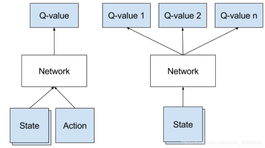
这就是深度学习的重点。神经网络非常擅长为高度结构化的数据提供良好的特性。 我们可以用神经网络来表示我们的Q函数，它将状态（四个游戏屏幕）和动作作为输入并输出相应的Q值。 或者，我们可以仅将游戏屏幕作为输入并输出每个可能动作的Q值。 这种方法的优点是，如果我们想要执行Q值更新或选择具有最高Q值的操作，我们只需要通过网络进行一次前向传递，并使所有操作的所有Q值立即可用。

This is the point, where deep learning steps in. Neural networks are exceptionally good in coming up with good features for highly structured data. We could represent our Q-function with a neural network, that takes the state (four game screens) and action as input and outputs the corresponding Q-value. Alternatively we could take only game screens as input and output the Q-value for each possible action. This approach has the advantage, that if we want to perform a Q-value update or pick the action with highest Q-value, we only have to do one forward pass through the network and have all Q-values for all actions immediately available.

DeepMind使用的网络架构如下:

Layer	Input	Filter size	Stride	Num filters	Activation	Output
conv1	84x84x4	8×8	4	32	ReLU	20×20×32
conv2	20×20×32	4×4	2	64	ReLU	9×9×64
conv3	9×9×64	3×3	1	64	ReLU	7×7×64
fc4	7×7×64			512	ReLU	512
fc5	512			18	Linear	18

这是一个经典的卷积神经网络，有三个卷积层，后面是两个完全连接的层。 熟悉对象识别网络的人可能会注意到没有池化层。 但如果你真的这么想，那么池化层就为你带来了一个平移不变性——网络变得对图像中对象的位置不敏感。 这对于像ImageNet这样的分类任务来说非常有意义，但对于游戏来说，球的位置对于确定潜在的奖励至关重要，我们不想丢弃这些信息！

This is a classical convolutional neural network with three convolutional layers, followed by two fully connected layers. People familiar with object recognition networks may notice that there are no pooling layers. But if you really think about that, then pooling layers buy you a translation invariance – the network becomes insensitive to the location of an object in the image. That makes perfectly sense for a classification task like ImageNet, but for games the location of the ball is crucial in determining the potential reward and we wouldn’t want to discard this information!

网络输入是四个84×84灰度游戏画面。 网络的输出是每个可能的动作的Q值（18 in Atari）。 Q值可以是任何实数值，这使得它成为回归任务，可以通过简单的平方误差损失进行优化。

Input to the network are four 84×84 grayscale game screens. Outputs of the network are Q-values for each possible action (18 in Atari). Q-values can be any real values, which makes it a regression task, that can be optimized with a simple squared error loss.

$L=\frac 1 2[\underbrace{r+\gamma max_{a'}Q(s',a')}_{\text{target}}-\underbrace{Q(s,a)}_{\text{prediction}}]^2$

对于给定的一个transition $<s，a，r，s'>$

1. 为当前状态执行前馈传递
2. 为下一个状态 $s'$做一个前馈传递 $max_{a'}Q(s',a')$
3. 将动作a的目标Q值设置为 $r +γmax_{a'}Q(s'，a')$（使用步骤2中计算的最大值）。 对于所有其他操作，将目标Q值设置为与步骤1中最初返回的相同，使这些输出的错误为0。
4. 使用反向传播更新权重。

---

Experience Replay 经验回放

---

现在我们已经知道了如何使用Q-learning估计每种状态下的未来回报，以及使用卷积神经网络逼近Q函数。但结果表明，用非线性函数逼近Q值并不十分稳定。有很多技巧可以让它收敛。而且它需要很长时间，几乎在一个GPU上一周。

By now we have an idea how to estimate the future reward in each state using Q-learning and approximate the Q-function using a convolutional neural network. But it turns out that approximation of Q-values using non-linear functions is not very stable. There is a whole bag of tricks that you have to use to actually make it converge. And it takes a long time, almost a week on a single GPU.

最重要的技巧是经验回放。 在游戏过程中，所有经验 $<s，a，r，s'>$都存储在回放存储器中。 在训练网络时，使用来自回放存储器的随机样本而不是最近的transition。 这打破了后续训练样本的相似性，否则可能将网络驱动到局部最小值。 经验回放使训练任务更加类似于通常的监督学习，这简化了调试和测试算法。 人们实际上可以收集人类游戏玩法和训练网络的所有这些经验。

---

Exploration-Exploitation

---

Q-learning试图解决信用分配问题 - 它会及时传播奖励，直到达到关键决策点，这是获得奖励的实际原因。 但我们还没有触及探索开发的困境…

Q-learning attempts to solve the credit assignment problem – it propagates rewards back in time, until it reaches the crucial decision point which was the actual cause for the obtained reward. But we haven’t touched the exploration-exploitation dilemma yet…

首先要注意的是，当Q-table或Q-network随机初始化时，其预测最初也是随机的。 如果我们选择具有最高Q值的动作，则动作将是随机的并且agent执行粗略的“探索”。 随着Q函数收敛，它返回更一致的Q值并且探索量减少。 可以这么说，Q-learning将探索作为算法的一部分。但这种探索是“贪婪的”，它采用了它发现的第一个有效策略。

Firstly observe, that when a Q-table or Q-network is initialized randomly, then its predictions are initially random as well. If we pick an action with the highest Q-value, the action will be random and the agent performs crude “exploration”. As a Q-function converges, it returns more consistent Q-values and the amount of exploration decreases. So one could say, that Q-learning incorporates the exploration as part of the algorithm. But this exploration is “greedy”, it settles with the first effective strategy it finds.

对上述问题的一个简单而有效的解决方法是 $ε-greedy$探索—概率 $ε$选择随机动作，否则采用具有最高Q值的“greedy”动作。 在他们的系统中，DeepMind实际上随着时间j将 $ε$从1减少到0.1 - 在开始时系统完全随机移动以最大限度地探索状态空间，然后它稳定下来到固定的探索速率。

A simple and effective fix for the above problem is ε-greedy exploration – with probability ε choose a random action, otherwise go with the “greedy” action with the highest Q-value. In their system DeepMind actually decreases ε over time from 1 to 0.1 – in the beginning the system makes completely random moves to explore the state space maximally, and then it settles down to a fixed exploration rate.

---

Deep Q-learning Algorithm

---

initialize replay memory D
initialize action-value function Q with random weights
observe initial state s
repeat
  select an action a
    with probability ε select a random action
    otherwise select a = argmaxa’Q(s,a’)
  carry out action a
  observe reward r and new state s’
  store experience <s, a, r, s’> in replay memory D
  sample random transitions <ss, aa, rr, ss’> from replay memory D
  calculate target for each minibatch transition
    if ss’ is terminal state then tt = rr
    otherwise tt = rr + γmaxa’Q(ss’, aa’)
  train the Q network using (tt - Q(ss, aa))^2 as loss
  s = s’
until terminated

DeepMind实际上还有很多技巧可以让它发挥作用 - 比如目标网络，错误剪辑，奖励裁剪等，但这些技巧超出了本次介绍的范围。

There are many more tricks that DeepMind used to actually make it work – like target network, error clipping, reward clipping etc, but these are out of scope for this introduction.

这个算法中最神奇的部分是它可以学习任何东西。 试想一下 - 因为我们的Q函数是随机初始化的，它最初会输出完整的垃圾。 我们正在使用这个垃圾（下一个状态的最大Q值）作为网络的目标，只是偶尔折叠一个微小的奖励。 这听起来很疯狂，它怎么能学到任何有意义的东西呢？ 事实是，确实如此。

The most amazing part of this algorithm is that it learns anything at all. Just think about it – because our Q-function is initialized randomly, it initially outputs complete garbage. And we are using this garbage (the maximum Q-value of the next state) as targets for the network, only occasionally folding in a tiny reward. That sounds insane, how could it learn anything meaningful at all? The fact is, that it does.