Python3抓取 深圳房地产均价数据，通过真实数据为购置不动产做决策分析（二）

接下来处理下之前收集到的房地产数据数据： 先分享一个学习数据预处理，数据挖掘，机器学习的实用网站：http://scikit-learn.org/stable/，有很多对应的教程。

之前收集数据文章的链接：http://www.cnblogs.com/ChrisInsistPy/p/9023477.html

本文中提到的数据清洗以及数据图形化都是通过pandas，以及matplotlib包等实现，通过学习一个比较有名的tutorial，来实现自己的小项目， tutorial地址：https://www.kaggle.com/c/house-prices-advanced-regression-techniques#tutorials

首先需要把存入MongoDB的数据读出来，直接读入pandas的DataFrame里，pandas包含了丰富的数据处理方法，下面会列举几个比较常用的，当然真正用的时候还是查文档比较好

从MongoDB读数据代码(相比之前的代码，对数据类型，表头稍作修改，具体请看Github源码)：

def load_data():
    try:
        client = MongoClient('localhost', 27017)  # connect db
        db = client['test']  # my db
        info = db['text_set']  # my collection
    except:
        print('connection error')

    data = pd.DataFrame(list(info.find()))  # find all data
    del data['_id']  # filter data
    dataset = data[['小区名称', '住房面积(平方米)', '平均价格(每平方)']]
    return dataset

 通过pd的DataFrame方法，可以把数据库中的数据读入data中，设置title后，去除数据库中的_id字段，然后返回dataset

pandas有很多对数据的操作，仅仅是列举：

def pandas_operations(dataset): # pandas基本操作
    dataset.info() #数据表基本信息
    dataset.dtypes #每一列的数据类型
    dataset.isnull() #拿到空值
    dataset['area'].unique() #看某一列的唯一值
    dataset.columns #查看列名称
    dataset.head() #前10行数据
    dataset.tail()
    dataset['column'].drop_duplicates() #删除重复值
    dataset['column'].replace('bj','test') #替换

通过seaborn包，这是一个简化了matlib操作的包，能简单的帮你生成漂亮的统计图

代码如下：

def kaggle_party(dataset): 
    print(dataset['平均价格(每平方)'].describe())
    dataset['平均价格(每平方)'] = pd.to_numeric(dataset['平均价格(每平方)'], errors='coerce') #转化为int
    mpl.rcParams['font.sans-serif'] = ['SimHei']
    sns.distplot(dataset['平均价格(每平方)']);
    plt.show()

注：在MongoDB中存储的数据是str类型的，所以要通过pandas的to_numeric()方法先将其转化为int类型

运行代码就生成统计图了：

我们会发现，大概平均的价格峰值在45000/平方米左右，但是我们会发现，极小值在6000-7000左右，而极大值在200000/平方左右，看似有些数据是不合理的，所以接下来我们会处理非合理数据。

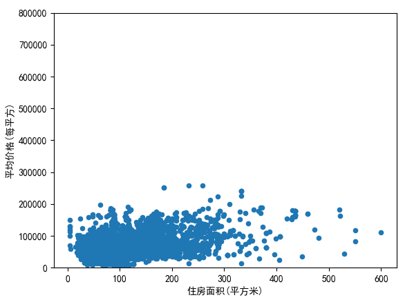
不过在处理之前，我们继续通过统计图来分析，接下来介绍一种scatter diagram 散点图，可以用来观测两个变量的关系以及偏离值，在收集的数据中，住房面积和均价可以说是老朋友了。 Tutorial的作者是这样说的：“One of the figures we may find interesting is the one between 'price' and 'area'. In this figure we can see the dots drawing a linear line, which almost acts like a border. It totally makes sense that the majority of the dots stay below that line. Basement areas can be equal to the above ground living area, but it is not expected a basement area bigger than the above ground living area (unless you're trying to buy a bunker).”

那么现在就用散点图来展示一下他们的关系：

代码如下：

def kaggle_party2(dataset):  # 散点状分布图
    var = '住房面积(平方米)'
    data = pd.concat([dataset['平均价格(每平方)'], dataset[var]], axis=1)
    mpl.rcParams['font.sans-serif'] = ['SimHei']
    data.plot.scatter(x=var, y='平均价格(每平方)', ylim=(0, 800000));
    plt.show()

运行结果如下：

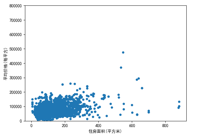
从这幅统计图中，发现了贫穷，真的可以限制你的想象力:-D, 还有超过50万/平米和大于800平米的房子，当然这些数据都不是我们要考虑的范围。因为我们要做的数据分析是根据大部分人的需求以及偏好为基础。所以，既然这么贵，删！！在清洗数据之前，首先继续对数据进行visualization。

接下来分析 Missing data

Missing data为在一个数据集里面，值为空的数据，因为我们抓取得数据都是百分百从html静态页面抓下来的，所以不存在null数据，但是我们还是需要验证一下：

代码如下：

def kaggle_party4(dataset): # check missing data and rates
    total = dataset.isnull().sum().sort_values(ascending=False)
    percent = (dataset.isnull().sum() / dataset.isnull().count().sort_values(ascending=False))
    missing_data = pd.concat([total, percent], axis=1, keys=['Total','Percent'])
    print(missing_data.head(20))
    # deal with missing data call drop

并且通过简单的运算，来算出null数据的比率，然后打印：

结果果然是，并没有null数据的存在：

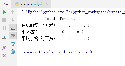
在tutorial中，如果某个column的空值数据的比率过高，就要采取一定的手段，去删除空值关联的其他column的数据，但是也要考虑到column之间的关系等。

接下来，进行 Univariate analysis

就是要设定一个中间标准值，然后查看偏离点的值的分布

代码如下：

def kaggle_party5(dataset): #consider the range of price deviation
    saleprice_scaled = StandardScaler().fit_transform(dataset['平均价格(每平方)'][:, np.newaxis]);
    low_range = saleprice_scaled[saleprice_scaled[:, 0].argsort()][:10]
    high_range = saleprice_scaled[saleprice_scaled[:, 0].argsort()][-10:]
    print('outer range (low) of the distribution:')
    print(low_range)
    print('\nouter range (high) of the distribution:')
    print(high_range)

运行后，得出的结果如下：

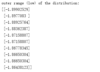
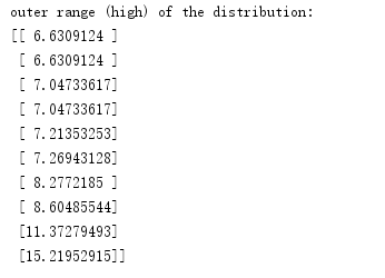
我们很明显的能发现，high of the distribution 对于标准值1的偏离度，明显大于low的值，尤其是10以上的偏离度，这是需要在数据处理中，需要被考虑的。

现在根据散点图，偏离分析等等得出的分析结果，我们需要删除一些偏离中心值过大的数据。我们准备把住房面积大于600的和平均价格大于30000的数据砍掉，代码如下：

def drop_data(dataset):
    dataset = dataset.drop(dataset[dataset['平均价格(每平方)'] > 300000].index)
    dataset = dataset.drop(dataset[dataset['住房面积(平方米)'] > 600].index)
    return dataset

然后我们再次用散点图表示出处理过的dataset：

可以发现，数据的分布更加的集中，更加的趋于合理化。

接下来

Who is 'SalePrice'?

我们已经对于房产售价做了很多分析，以及数据清理。So now it's time to go deep and understand how 'SalePrice' complies with the statistical assumptions that enables us to apply multivariate techniques.

从统计学的角度来看问题：引用Hair et al. (2013) 提出的四个标准

1.Normality ：数据应该遵循自然分配

2.Homoscedasticity ：假设依赖数值的元素是在预测范围之内

3.Linearity：利用散点图去找线性规律

4.Absence of correlated errors：错误之间的一致性关系

 

接下来我们测试显示一下，清洗过后的数据显示的峰度图，偏态分布

如图所示：

好吧，看起来，图形化的信息并没有像我们预料到的normal distribution，在tutorial作者的提示下，我们试着用统计学书上提到最常用的，把斜率变得更加positive，用log！

代码如下：

def kaggle_party7(dataset):
    # histogram and normal probability plot
    mpl.rcParams['font.sans-serif'] = ['SimHei']
    dataset['平均价格(每平方)'] = np.log(dataset['平均价格(每平方)']) #log
    sns.distplot(dataset['平均价格(每平方)'], fit=norm);
    fig = plt.figure()
    res = stats.probplot(dataset['平均价格(每平方)'], plot=plt)
    plt.show()

运行结果如下：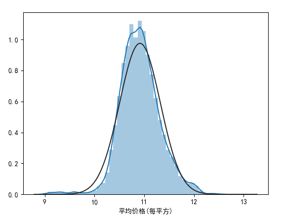

我们会惊喜的发现运用了这种数据转换的方式，满足了我们的需求！log在统计学中，可以避免极值的出现，从而使得分布更加趋于Normality。

完整代码请参考(包括抓取数据代码)：https://github.com/wy9884255/src

数据分析整体代码如下：

  1 #invite people for the Kaggle party
  2 import pandas as pd
  3 import numpy as np
  4 import seaborn as sns
  5 import matplotlib as mpl
  6 from scipy.stats import norm
  7 from scipy import stats
  8 from sklearn.preprocessing import StandardScaler
  9 import warnings
 10 import matplotlib.pyplot as plt
 11 from pymongo import MongoClient
 12 warnings.filterwarnings('ignore')
 13 
 14 
 15 def load_data():
 16     try:
 17         client = MongoClient('localhost', 27017)  # connect db
 18         db = client['test']  # my db
 19         info = db['text_set']  # my collection
 20     except:
 21         print('connection error')
 22 
 23     data = pd.DataFrame(list(info.find()))  # find all data
 24     del data['_id']  # filter data
 25     dataset = data[['小区名称', '住房面积(平方米)', '平均价格(每平方)']]
 26     return dataset
 27 
 28 
 29 def pandas_operations(dataset): # pandas基本操作
 30     dataset.info() #数据表基本信息
 31     dataset.dtypes #每一列的数据类型
 32     dataset.isnull() #拿到空值
 33     dataset['area'].unique() #看某一列的唯一值
 34     dataset.columns #查看列名称
 35     dataset.head() #前10行数据
 36     dataset.tail()
 37     dataset['column'].drop_duplicates() #删除重复值
 38     dataset['column'].replace('bj','test') #替换
 39 
 40 
 41 def kaggle_party1(dataset): # 线图加直方图
 42     print(dataset['平均价格(每平方)'].describe())
 43     mpl.rcParams['font.sans-serif'] = ['SimHei']
 44     sns.distplot(dataset['平均价格(每平方)']);
 45     plt.show()
 46 
 47 def kaggle_party2(dataset):  # 散点状分布图
 48     var = '住房面积(平方米)'
 49     data = pd.concat([dataset['平均价格(每平方)'], dataset[var]], axis=1)
 50     mpl.rcParams['font.sans-serif'] = ['SimHei']
 51     data.plot.scatter(x=var, y='平均价格(每平方)', ylim=(0, 800000));
 52     plt.show()
 53 
 54 def kaggle_party3(dataset):
 55     k = 10  # number of variables for heatmap
 56     corrmat = dataset.corr()
 57     cols = corrmat.nlargest(k, '平均价格(每平方)')['平均价格(每平方)'].index
 58     mpl.rcParams['font.sans-serif'] = ['SimHei']
 59     cm = np.corrcoef(dataset[cols].values.T)
 60     sns.set(font_scale=1.25)
 61     hm = sns.heatmap(cm, cbar=True, annot=True, square=True, fmt='.2f', annot_kws={'size': 10}, yticklabels=cols.values,
 62                      xticklabels=cols.values)
 63     plt.show()
 64 
 65 
 66 def kaggle_party4(dataset): # check missing data and rates
 67     total = dataset.isnull().sum().sort_values(ascending=False)
 68     percent = (dataset.isnull().sum() / dataset.isnull().count().sort_values(ascending=False))
 69     missing_data = pd.concat([total, percent], axis=1, keys=['Total','Percent'])
 70     print(missing_data.head(20))
 71     # deal with missing data call drop
 72 
 73 
 74 def kaggle_party5(dataset): #consider the range of price deviation
 75     saleprice_scaled = StandardScaler().fit_transform(dataset['平均价格(每平方)'][:, np.newaxis]);
 76     low_range = saleprice_scaled[saleprice_scaled[:, 0].argsort()][:10]
 77     high_range = saleprice_scaled[saleprice_scaled[:, 0].argsort()][-10:]
 78     print('outer range (low) of the distribution:')
 79     print(low_range)
 80     print('\nouter range (high) of the distribution:')
 81     print(high_range)
 82 
 83 def kaggle_party6(dataset):
 84     # histogram and normal probability plot
 85     mpl.rcParams['font.sans-serif'] = ['SimHei']
 86     sns.distplot(dataset['平均价格(每平方)'], fit=norm);
 87     fig = plt.figure()
 88     res = stats.probplot(dataset['平均价格(每平方)'], plot=plt)
 89     plt.show()
 90 
 91 
 92 def kaggle_party7(dataset):
 93     # histogram and normal probability plot
 94     mpl.rcParams['font.sans-serif'] = ['SimHei']
 95     dataset['平均价格(每平方)'] = np.log(dataset['平均价格(每平方)']) #log
 96     sns.distplot(dataset['平均价格(每平方)'], fit=norm);
 97     fig = plt.figure()
 98     res = stats.probplot(dataset['平均价格(每平方)'], plot=plt)
 99     plt.show()
100 
101 
102 def kaggle_party8(dataset):
103     # using normality data
104     mpl.rcParams['font.sans-serif'] = ['SimHei']
105     dataset['平均价格(每平方)'] = np.log(dataset['平均价格(每平方)']) #log
106     plt.scatter(dataset['住房面积(平方米)'], dataset['平均价格(每平方)']);
107     plt.show()
108 
109 
110 def drop_data(dataset):
111     dataset = dataset.drop(dataset[dataset['平均价格(每平方)'] > 300000].index)
112     dataset = dataset.drop(dataset[dataset['住房面积(平方米)'] > 600].index)
113     return dataset
114 
115 
116 def main():
117     dataset = load_data()
118     dataset['住房面积(平方米)'] = pd.to_numeric(dataset['住房面积(平方米)'], errors='coerce')# convert str to int
119     dataset['平均价格(每平方)'] = pd.to_numeric(dataset['平均价格(每平方)'], errors='coerce')# convert str to int
120     # kaggle_party1(dataset)
121     # kaggle_party2(dataset)
122     # kaggle_party3(dataset)
123     # kaggle_party4(dataset)
124     # kaggle_party5(dataset)
125 
126     #data has been cleaned
127     # dataset = drop_data(dataset)
128     # kaggle_party2(dataset)
129     # kaggle_party6(dataset)
130     # kaggle_party7(dataset)
131     kaggle_party8(dataset)
132 
133 
134 if __name__ == '__main__':
135     main()