《DSP using MATLAB》Problem 8.14

代码：

%% ------------------------------------------------------------------------
%%            Output Info about this m-file
fprintf('\n***********************************************************\n');
fprintf('        <DSP using MATLAB> Problem 8.14 \n\n');

banner();
%% ------------------------------------------------------------------------

Wp = 10; Ws = 15; Rp = 1; As = 50;
Fp = Wp/(2*pi);
Fs = Ws/(2*pi);

Ripple = 10 ^ (-Rp/20)
Attn = 10 ^ (-As/20)

% Analog filter design:
[b, a] = afd('cheby1', Fp, Fs, Rp, As);
%[b, a] = afd_chb1(Wp, Ws, Rp, As);

% Calculation of second-order sections:
[C, B, A] = sdir2cas(b, a);

% Calculation of Frequency Response:
[db, mag, pha, ww] = freqs_m(b, a, 20);

% Calculation of Impulse Response:
[ha, x, t] = impulse(b, a);


%% -------------------------------------------------
%%                    Plot
%% -------------------------------------------------  

figure('NumberTitle', 'off', 'Name', 'Problem 8.14 Analog Chebyshev-I lowpass')
set(gcf,'Color','white'); 
M = 1.0;                          % Omega max

subplot(2,2,1); plot(ww, mag);  grid on; axis([-20, 20, 0, 1.2]);
xlabel(' Analog frequency in rad/sec units'); ylabel('|H|'); title('Magnitude in Absolute');
set(gca, 'XTickMode', 'manual', 'XTick', [-15, -10, 0, 10, 15]);
set(gca, 'YTickMode', 'manual', 'YTick', [0, 0.003, 0.89, 1]);

subplot(2,2,2); plot(ww, db);  grid on; %axis([0, M, -50, 10]);
xlabel('Analog frequency in rad/sec units'); ylabel('Decibels'); title('Magnitude in dB ');
set(gca, 'XTickMode', 'manual', 'XTick', [-15, -10, 0, 10, 15]);
set(gca, 'YTickMode', 'manual', 'YTick', [-50, -1, 0]);
set(gca,'YTickLabelMode','manual','YTickLabel',['50';' 1';' 0']);

subplot(2,2,3); plot(ww, pha/pi);  grid on; axis([-20, 20, -1.2, 1.2]);
xlabel('Analog frequency in rad/sec nuits'); ylabel('radians'); title('Phase Response');
set(gca, 'XTickMode', 'manual', 'XTick', [-15, -10, 0, 10, 15]);
set(gca, 'YTickMode', 'manual', 'YTick', [-1:0.5:1]);


subplot(2,2,4); plot(t, ha); grid on; %axis([0, 30, -0.05, 0.25]); 
xlabel('time in seconds'); ylabel('ha(t)'); title('Impulse Response');

　　运行结果：

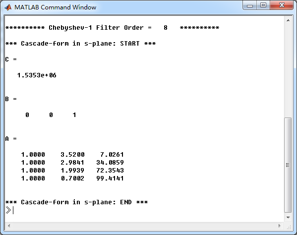
       通带、阻带绝对指标

        模拟Chebyshev-1型低通滤波器串联形式系数

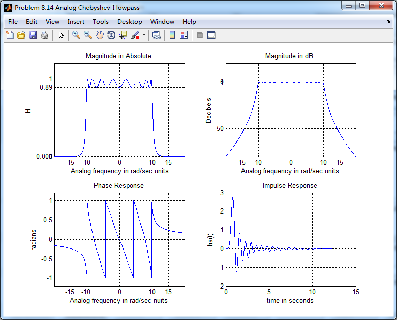
        幅度谱、相位谱和脉冲响应

       将通带部分放大，如下图

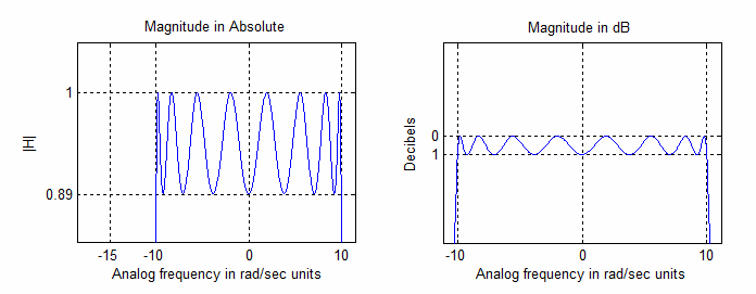
        依chebyshev-1型低通特征可知，只是通带部分有振荡，图也显示了这点。