Chapter 2 Rigid Body Motion
A rigid motion of an object is a motion which preserves distance between points. The study of robot kinematics, dynamics, and control has at its heart the study of the motion of rigid objects. In this chapter, we provide a description of rigid body motion using the tools of linear algebra and screw theory.
Chasles proved that a rigid body can be moved from any one position to any other by a movement consisting of rotation about a straight line followed by translation parallel to that line. This motion is what we refer to in this book as a screw motion.
The infinitesimal version of a screw motion is called a twist and it provides a description of the instantaneous velocity of a rigid body in terms of its linear and angular components. Screws and twists play a central role in our formulation of the kinematics of robot mechanisms.
Any system of forces acting on a rigid body can be replaced by a single force applied along a line, combined with a torque about that same line. Such a force is referred to as a wrench. Wrenches are dual to twists, so that many of the theorems which apply to twists can be extended to wrenches.
In this chapter, we present a more modern treatment of the theory of screws based on linear algebra and matrix groups. The fundamental tools are the use of homogeneous coordinates to represent rigid motions and the matrix exponential, which maps a twist into the corresponding screw motion.
There are two main advantages to using screws, twists, and wrenches for describing rigid body kinematics. The first is that they allow a global description of rigid body motion which does not suffer from singularities due to the use of local coordinates. Such singularities are inevitable when one chooses to represent rotation via Euler angles, for example. The second advantage is that screw theory provides a very geometric description of rigid motion which greatly simplifies the analysis of mechanisms.
1 Rigid Body Transformations
The motion of a particle moving in Euclidean space is described by giving the location of the particle at each instant of time, relative to an inertial Cartesian coordinate frame. Specifically, we choose a set of three orthonormal axes and specify the particle’s location using the triple , where each coordinate gives the projection of the particle’s location onto the corresponding axis. A trajectory of the particle is represented by the parameterized curve .
In robotics, we are frequently interested not in the motion of individual particles, but in the collective motion of a set of particles, such as the link of a robot manipulator. To this end, we loosely define a perfectly rigid body as a completely “undistortable” body. More formally, a rigid body is a collection of particles such that the distance between any two particles remains fixed, regardless of any motions of the body or forces exerted on the body. Thus, if p and q are any two points on a rigid body then, as the body moves, p and q must satisfy
A rigid motion of an object is a continous movement of the particles in the object such that the distance between any two particles remains fixed at all times. The net movement of a rigid body from one location to another via a rigid motion is called a rigid displacement. In general, a rigid displacement may consist of both translation and rotation of the object.
Given an object described as a subset of , a rigid motion of an object is represented by a continuous family of mappings which describe how individual points in the body move as a function of time, relative to some fixed Cartesian coordinate frame. That is, if we move an object along a continuous path, g(t) maps the initial coordinates of a point on the body to the coordinates of that same point at time t. A rigid displacement is represented by a single mapping which maps the coordinates of points in the rigid body from their initial to final configurations.
Given two points , the vector connecting to is defined to be the directed line segment going from to . In coordinates this is given by with . Though both points and vectors are represented by 3-tuples of numbers, they are conceptually quite different. A vector has a direction and a magnitude. (By the magnitude of a vector, we will mean its Euclidean norm, i.e., .) It is, however, not attached to the body, since there may be other pairs of points on the body, for instance and with , for which the same vector v also connects r to s. A vector is sometimes called a free vector to indicate that it can be positioned anywhere in space without changing its meaning.
The action of a rigid transformation on points induces an action on vectors in a natural way. If we let
represent a rigid displacement, then vectors transform according to
Note that the right-hand side is the difference of two points and is hence also a vector.
Since distances between points on a rigid body are not altered by rigid motions, a necessary condition for a mapping to describe a rigid motion is that distances be preserved by the mapping. However, this condition is not sufficient since it allows internal reflections, which are not physically realizable. That is, a mapping might preserve distance but not preserve orientation. For example, the mapping preserves distances but reflects points in the body about the xy plane. To eliminate this possibility, we require that the cross product between vectors in the body also be preserved. We will collect these requirements to define a rigid body transformation as a mapping from to which represents a rigid motion:
Definition 2.1. Rigid body transformation
A mapping is a rigid body transformation if it satisfies the following properties:
- Length is preserved: for all points
- The cross product is preserved: for all vectors .
There are some interesting consequences of this definition. The first is that the inner product is preserved by rigid body transformations. One way to show this is to use the polarization identity,
and the fact that
to conclude that for any two vectors
,
In particular, orthogonal vectors are transformed to orthogonal vectors. Coupled with the fact that rigid body transformations also preserve the cross product (property 2 of the definition above), we see that rigid body transformations take orthonormal coordinate frames to orthonormal coordinate frames.
The fact that the distance between points and cross product between vectors is fixed does not mean that it is inadmissible for particles in a rigid body to move relative to each other, but rather that they can rotate but not translate with respect to each other. Thus, to keep track of the motion of a rigid body, we need to keep track of the motion of any one particle on the rigid body and the rotation of the body about this point. In order to do this, we represent the configuration of a rigid body by attaching a Cartesian coordinate frame to some point on the rigid body and keeping track of the motion of this body coordinate frame relative to a fixed frame. The motion of the individual particles in the body can then be retrieved from the motion of the body frame and the motion of the point of attachment of the frame to the body. We shall require that all coordinate frames be right-handed: given three orthonormal vectors which define a coordinate frame, they must satisfy .
Since a rigid body transformation preserves the cross product, right-handed coordinate frames are transformed to right-handed coordinate frames. The action of a rigid transformation on the body frame describes how the body frame rotates as a consequence of the rigid motion. More precisely, if we describe the configuration of a rigid body by the right-handed frame given by the vectors attached to a point , then the configuration of the rigid body after the rigid body transformation g is given by the right-handed frame of vectors attached to the point .
2 Rotational Motion in

We begin the study of rigid body motion by considering, at the outset, only the rotational motion of an object. We describe the orientation of the body by giving the relative orientation between a coordinate frame attached to the body and a fixed or inertial coordinate frame. From now on, all coordinate frames will be right-handed unless stated otherwise. Let A be the inertial frame, B the body frame, and
the coordinates of the principal axes of B relative to A (see Figure 2.1). Stacking these coordinate vectors next to each other, we define a 3 × 3 matrix:
We call a matrix constructed in this manner a rotation matrix: every rotation of the object relative to the ground corresponds to a matrix of this form.
2.1 Properties of rotation matrices
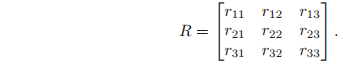
A rotation matrix has two key properties that follow from its construction. Let
be a rotation matrix and
be its columns. Since the columns of R are mutually orthonormal, it follows that

As conditions on the matrix R, these properties can be written as
From this it follows that
To determine the sign of the determinant of
, we recall from linear algebra that
Since the coordinate frame is right-handed, we have that
so that
.
The set of all 3 × 3 matrices which satisfy these two properties is denoted
. The notation
abbreviates special orthogonal. Special refers to the fact that
rather than ±1.
More generally, we may define the space of rotation matrices in
by
is a group under the operation of matrix multiplication. A set G together with a binary operation ◦ defined on elements of G is called a group if it satisfies the following axioms:
- Closure: If , then .
- Identity: There exists an identity element, e, such that for every .
- Inverse: For each , there exists a (unique) inverse, , such that .
- Associativity: If g1, g2, g3 ∈ G, then (g1 ◦ g2) ◦ g3 = g1 ◦ (g2 ◦ g3).
We refer to as the rotation group of .
Every configuration of a rigid body that is free to rotate relative to a fixed frame can be identified with a unique . Under this identification, the rotation group is referred to as the configuration space of the system and a trajectory of the system is a curve for . More generally, we shall call a set a configuration space for a system if every element corresponds to a valid configuration of the system and each configuration of the system can be identified with a unique element of .
A rotation matrix
also serves as a transformation, taking coordinates of a point from one frame to another. Consider the point q shown in Figure 2.1. Let
be the coordinates of
relative to frame B. The coordinates of
relative to frame A can be computed as follows: since
are projections of q onto the coordinate axes of B, which, in turn, have coordinates
with respect to A, the coordinates of
relative to frame A are given by
This can be rewritten as
In other words, , when considered as a map from to , rotates the coordinates of a point from frame B to frame A.
The action of a rotation matrix on a point can be used to define the action of the rotation matrix on a vector. Let
be a vector in the frame B defined as
. Then,
Since matrix multiplication is linear, it may be verified that if
then we still have that
and hence the action of
on a vector is well defined.
.
Rotation matrices can be combined to form new rotation matrices using matrix multiplication. If a frame C has orientation
relative to a frame B, and B has orientation
relative to another frame A, then the orientation of C relative to A is given by
.
$R_{ac}, when considered as a map from
to \mathbb R^3$, rotates the coordinates of a point from frame C to frame A by first rotating from C to B and then
from B to A. Equation is the composition rule for rotations.
A rotation matrix represents a rigid body transformation in the sense of the definition of the previous section. This is to say, it preserves distance and orientation. We prove this using some algebraic properties of the cross product operation between two vectors. Recall that the cross product between two vectors
is defined as
Since the cross product by a is a linear operator,
may be represented using a matrix. Defining
we can write
We will often use the notation ba as a replacement for (a)∧.
Lemma 2.1. Given
and
, the following properties hold:
The first property in the lemma asserts that rotation by the matrix R commutes with the cross product operation; that is, the rotation of the cross product of two vectors is the cross product of the rotation of each of the vectors by R. The second property has an interpretation in terms of rotation of an instantaneous axis of rotation, which will become clear shortly. For now, we will merely use it as an algebraic fact. The proof of the lemma is by calculation.
Proposition 2.2. Rotations are rigid body transformations
A rotation is a rigid body transformation; that is,
- R preserves distance: for all .
- R preserves orientation:
for all
.
Proof. Property 1 can be verified by direct calculation:
.
Property 2 follows from equation.

2.2 Exponential coordinates for rotation
A common motion encountered in robotics is the rotation of a body about a given axis by some amount. Let be a unit vector which specifies the direction of rotation and let be the angle of rotation in radians. Since every rotation of the object corresponds to some , we would like to write as a function of and .
To motivate our derivation, consider the velocity of a point q attached to the rotating body. If we rotate the body at constant unit velocity about the axis
, the velocity of the point,
, may be written as
This is a time-invariant linear differential equation which may be integrated to give
where q(0) is the initial (t = 0) position of the point and eωt b is the matrix exponential

It follows that if we rotate about the axis
at unit velocity for
units of time, then the net rotation is given by
From its definition, it is easy to see that the matrix
is a skew-symmetric matrix, i.e., it satisfies
. The vector space of all 3 × 3 skew matrices is denoted so(3) and more generally the space of n × n skew-symmetric matrices is
The set is a vector space over the reals. Thus, the sum of two elements of is an element of and the scalar multiple of any element of is an element of . Furthermore, we can identify with using the relationship (2.4) and the fact .
It will be convenient to represent a skew-symmetric matrix as the product of a unit skew-symmetric matrix and a real number. Given a matrix
,
, and a real number
, we write the exponential of
as

Equation (2.11) is an infinite series and, hence, not useful from a computational standpoint. To obtain a closed-form expression for exp(
), we make use of the following formulas for powers of
, which are verified by direct calculation.
Lemma 2.3. Given
, the following relations hold:

and higher powers of
can be calculated recursively.

and hence
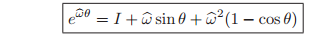
This formula, commonly referred to as Rodrigues’ formula, gives an efficient method for computing exp(
). When
, it may be verified (see Exercise 12) that

We now verify that exp(
) is indeed a rotation matrix.
Proposition 2.4. Exponentials of skew matrices are orthogonal
Given a skew-symmetric matrix
and
,
Proof. Defining
, we must verify that
and
. To verify the first property, we have the following chain of equalities, which can be checked using equation (2.14),
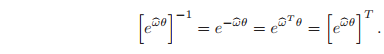
Proposition 2.4 asserts that the exponential map transforms skewsymmetric matrices into orthogonal matrices. Geometrically, the skewsymmetric matrix corresponds to an axis of rotation (via the mapping
) and the exponential map generates the rotation corresponding to rotation about the axis by a specified amount θ. Every rotation matrix can be represented as the matrix exponential of some skew-symmetric matrix; that is, the map exp : so(3) → SO(3) is surjective (onto).
Proposition 2.5. The exponential map is surjective onto
Given
, there exists
,
and
such that
exp(
).
Proof. The proof is constructive. We equate terms of
and exp(
) and solve the corresponding equations. By way of notation, we have the rotation matrix
to be
Defining
, write equation
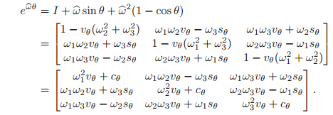
Proposition 2.5. The exponential map is surjective onto
Given
, there exists
and
such that
exp(
).
Equating (2.15) with (2.16), we see that

To verify that this equation has a solution, we recall that the trace of R is equal to the sum of its eigenvalues. Since R preserves lengths and
, its eigenvalues have magnitude 1 and occur in complex conjugate pairs (see Exercise 3). It follows that
and hence we can set
Note that there is an ambiguity in the value of
, in the sense that
or
could be chosen as well.
Now, equating the off-diagonal terms of
and exp(
), we get
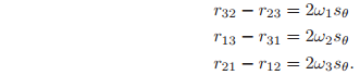
If
, we choose

Indeed, the exponential map is a many-to-one map from KaTeX parse error: Expected group after '\mathbb' at position 10: R\mathbb ^̲3 onto
. If
, then
and hence
and
can be chosen arbitrarily. If
, the above construction shows that there are two distinct
and
such that
exp(
).
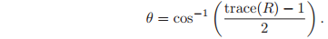
The components of the vector are called the exponential coordinates for . Considering to be an axis of rotation with unit magnitude and to be an angle, Propositions 2.4 and 2.5 combine to give the following classic theorem.
Theorem 2.6 (Euler). Any orientation is equivalent to a rotation about a fixed axis through an angle .
This method of representing a rotation is also known as the equivalent axis representation. We note from the preceding proof that this representation is not unique since choosing and gives the same rotation as and . Furthermore, if we insist that ω have unit magnitude, then is arbitrary for (by choosing ). The former problem is a consequence of the exponential map being many-to-one and the latter is referred to as a singularity of the equivalent axis representation, alluding to the fact that one may lose smooth dependence of the equivalent axis as a function of the orientation at .
2.3 Other representations
The exponential coordinates are called the canonical coordinates of the rotation group.
Euler angles
One method of describing the orientation of a coordinate frame B relative to another coordinate frame A is as follows: start with frame B coincident with frame A. First, rotate the B frame about the z-axis of frame B (at this time coincident with frame A) by an angle , then rotate about the (new) y-axis of frame B by an angle , and then rotate about the (once again, new) z-axis of frame B by an angle . This yields a net orientation and the triple of angles is used to represent the rotation.
The angles
are called the ZYZ Euler angles. Since all rotations are performed about the principal axes of the moving frame, we define the following elementary rotations about the x-, y-, and z-axes:

To derive the final orientation of frame B, it is easiest to derive the formula by viewing the rotation with B considered as the fixed frame, since then all rotations then occur around fixed axes. The appropriate sequence of rotations for the frame A, considering the B frame as fixed, is

Inverting this expression gives the rotation matrix of B relative to A:

Here
,
are abbreviations for
and
, respectively, and similarly for the other terms.
It is clear that any matrix of the form in equation (2.19) is an orthogonal matrix (since it is a composition of elementary rotations). As in the case of the exponential map, the converse question of whether the map from
is surjective is an important one. The answer to this question is affirmative: given a rotation
, the Euler angles can be computed by solving equation (2.19) for
,
, and
. For example, when sin
, the solutions are

where
computes
but uses the sign of both x and y to determine the quadrant in which the resulting angle lies.
ZYZ Euler angles are an example of a local parameterization of SO(3). As in the case of the equivalent axis representation, singularities in the parameterization (referring to the lack of existence of global, smooth solutions to the inverse problem of determining the Euler angles from the rotation) occur at , the identity rotation. In particular, we note that of the form yields . Thus, there are infinitely many representations of the identity rotation in the ZYZ Euler angles parameterization.
Other types of Euler angle parameterizations may be devised by using different ordered sets of rotation axes. Common choices include ZYX axes (Fick angles) and YZX axes (Helmholtz angles). The ZYX Euler angles are also referred to as the yaw, pitch, and roll angles, with Rab defined by rotating about the x-axis in the body frame (roll), then the y-axis in the body frame (pitch), and finally the z-axis in the body frame (yaw). Both the ZYX and YZX Euler angle parameterizations have the advantage of not having a singularity at the identity orientation,
, though they do contain singularities at other, different, orientations. For example, in the instance of ZYX Euler angles, we have:

which is singular when θ = −π/2. It is a fundamental topological fact that singularities can never be eliminated in any 3-dimensional representation of SO(3). This situation is similar to that of attempting to find a global coordinate chart on a sphere, which also fails.
Quaternions
Quaternions generalize complex numbers and can be used to represent rotations in much the same way as complex numbers on the unit circle can be used to represent planar rotations. Unlike Euler angles, quaternions give a global parameterization of , at the cost of using four numbers instead of three to represent a rotation.
Formally, a quaternion is a vector quantity of the form

where
is the scalar component of
and
is the vector component. A convenient shorthand notation is Q = (q0,~q ) with
. The set of quaternions
is a 4-dimensional vector space over the reals and forms a group with respect to quaternion multiplication, denoted “·”. Multiplication is distributive and associative, but not commutative; it satisfies the relations
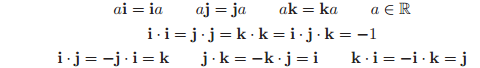
The conjugate of a quaternion
is given by
and the magnitude of a quaternion satisfies

It is straightforward to verify that the inverse of a quaternion is
and that
is the identity element for quaternion multiplication.
The product between two quaternions has a simple form in terms of the inner and cross products between vectors in
. Let
and
be quaternions, where
are the scalar parts of
and
and
are the vector parts. It can be shown algebraically that the product of two quaternions satisfies:

In most applications, this formula eliminates the need to make direct use of the multiplicative relations given above.
The unit quaternions are the subset of all
such that
. The unit quaternions also form a group with respect to quaternion multiplication (Exercise 6). Given a rotation matrix
exp(
), we define the associated unit quaternion as

where
represents the unit axis of rotation and
represents the angle of rotation. A detailed calculation shows that if
represents a rotation between frame A and frame B, and
represents a rotation between frames B and C, then the rotation between A and C is given by the quaternion

Thus, the group operation on unit quaternions directly corresponds to the group operation for rotations. Given a unit quaternion
, we can extract the corresponding rotation by setting
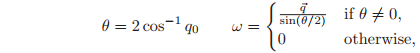
and
exp(
).
Since the group structure for quaternions directly corresponds to that of rotations, quaternions provide an efficient representation for rotations which do not suffer from singularities.
reference
A Mathematical Introduction to Robotic Manipulation Richard M. Murray, Zexiang Li, S. Shankar Sastry