一：SIFT算法的特征原理描述

SIFT算法在图像尺度空间基础上，实现了对图像缩放、旋转保持不变性的图像局部特征的描述。实质可以归为在不同尺度空间上查找特征点（关键点）的问题。SIFT算法实现特征匹配的基本流程如下：

1. 尺度空间的搭建

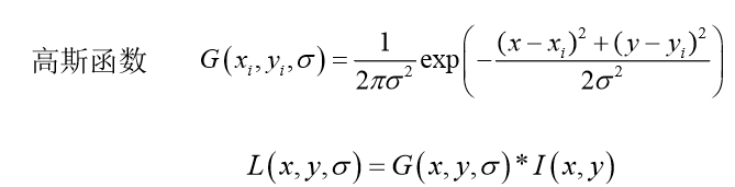
首先引入尺度空间的概念：它可以模拟人在距离目标由近到远的过程中，目标在视网膜当中形成图像的过程，尺度越大越模糊，相当于我们观察远处的物体。如果需要识别出包含不同尺寸的同一物体的两幅图像，随着物体在图像中大小发生变化，属于该物体的局部区域的大小也会发生变化。SIFT算法采用高斯图像金字塔，对图像做高斯平滑和降采样，一幅图像可以产生几组图像，一组图像包括几层图像，从而实现尺度的连续性。高斯核是唯一可以产生多尺度空间的核，一个图像的尺度空间，L(x, y, σ) ,定义为原始图像 I(x, y)与一个可变尺度的2 维高斯函数G(x, y, σ) 卷积运算。

尺度归一化的高斯拉普拉斯算子能够得到最稳定的图像特征，但因为计算量太大，所以引入了高斯差分金字塔（DOG），DoG在计算上只需相邻高斯平滑后图像相减，即高斯差分金字塔的第1组第1层是由高斯金字塔的第1组第2层减第1组第1层得到的，以此类推，逐组逐层生成每一个差分图像，所有差分图像构成差分金字塔，每一组在层数上，高斯差分金字塔比高斯金字塔少一层，从而简化了计算。

2. DOG局部极值检测

SIFT特征点是由DOG空间的局部极值点组成的。为了寻找DoG函数的极值点，将每一个像素点和它所有的相邻点进行比较。如图所示，将中间带叉号的检测点和它同尺度的8个相邻点和上下相邻尺度对应的9×2个点，即2*9+8=26，这26个像素点进行比较，若在这26个领域中是最大或最小值时，就认为该点是图像在该尺度下一个候选的特征点。

3. 对上一过程中得出的候选极值点进行筛选，去除边缘响应点，得到真正的特征点

DoG函数的峰值点在边缘方向有较大的主曲率，而在垂直边缘的方向有较小的主曲率。SIFT寻找的局部图像块，期望局部块中的主梯度方向与其他方向的梯度相差不要太大，通过计算DOG的二阶导数（Hessian矩阵），得到主梯度方向和其他方向的比值，保留该比值小于一定数值的局部特征点。主曲率可以通过计算在该点位置尺度的2×2的Hessian矩阵得到，导数由采样点相邻差来估计：

D 表示DOG金字塔中某一尺度的图像x方向求导两次

D的主曲率和H的特征值成正比。令 α ，β为特征值，则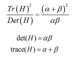

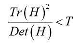时保留关键点，反之剔除

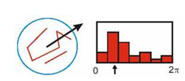
4. 特征点方向匹配

为了实现旋转不变形，基于每个点周围梯度的方向和大小，SIFT算法引入了主方向描述参考方向，主方向使用方向直方图来衡量。

5.关键特征点的描述

其中描述子由2×2×8维向量表征，也即是 2×2个8方向的方向直方图组成。左图的种子点由8×8单元组成。每一个小格都代表了特征点邻域所在的尺度空间的一个像素，箭头方向代表了像素梯度方向，箭头长度代表该像素的幅值。然后在4×4的窗口内计算8个方向的梯度方向直方图。绘制每个梯度方向的累加可形成一个种子点。

6. 通过特征点的两两比较，找出相互匹配的若干个特征点，建立对应的关系

关键点的匹配可以采用穷举法来完成，但是这样耗费的时间太多，一般都采用kd树的数据结构来完成搜索。搜索的内容是以目标图像的关键点为基准，搜索与目标图像的特征点最邻近的原图像特征点和次邻近的原图像特征点。

二：分别运用SIFT和Harris算法，实现图像的特征提取

使用开源工具包VLFeat提供的二进制文件来计算图像的SIFT特征。VLFeat工具包可以从http://www.vlfeat.org/下载，二进制文件可以在所有主要的平台上运行。将下载后的VLFeat解压，选择适合你电脑的位数。注意！！！官网上是最新的VLfeat-0.9.21版本，但最好选择VLfeat-0.9.20版本，如果用最新版本，有的电脑会出现生成的picture1.sift文件为空的情况，导致报错picture1.sift not found

例如我的电脑是64位，所以选用win64，并将其拷贝在我想要的目录下，然后在sift.py下，将cmmd中的目录修改为你自己放置的Vlfeat bin所在目录，注意！！！ 绝对路径的后面要加一个空格，否则也会报错找不到sift文件

由于该二进制文本需要的图像格式为灰度.pgm，所以首先将其转换成.pgm格式文件，如下图所示：

每一行的前四个数值依次表示兴趣点的横纵坐标，尺度和方向角度，后面紧接者的是对应描述符的128维向量。

通过read_features_from_file函数读取特征属性值，然后将其以矩阵的形式返回，由Numpy库中的loadtxt()函数来处理这所有的工作。若要修改描述子，可以通过savetxt()函数来实现，它的参数hstack()函数通过拼接不同的行向量来实现水平堆叠两个向量的功能。读取特征后，使用函数draw_circle()函数绘制出圆圈，实现可视化。

test1.py

# -*- coding: utf-8 -*-
from PIL import Image
from pylab import *
from PCV.localdescriptors import sift
from PCV.localdescriptors import harris

# 添加中文字体支持
from matplotlib.font_manager import FontProperties
font = FontProperties(fname=r"c:\windows\fonts\SimSun.ttc", size=14)

imname = 'picture1.jpg'
im = array(Image.open(imname).convert('L'))
sift.process_image(imname, 'picture1.sift')
l1, d1 = sift.read_features_from_file('picture1.sift')

figure()
gray()
subplot(131)
sift.plot_features(im, l1, circle=False)
title(u'SIFT特征',fontproperties=font)
subplot(132)
sift.plot_features(im, l1, circle=True)
title(u'用圆圈表示SIFT特征尺度',fontproperties=font)

# 检测harris角点
harrisim = harris.compute_harris_response(im)

subplot(133)
filtered_coords = harris.get_harris_points(harrisim, 6, 0.1)
imshow(im)
plot([p[1] for p in filtered_coords], [p[0] for p in filtered_coords], '*')
axis('off')
title(u'Harris角点',fontproperties=font)

show()

sift.py

from PIL import Image
import os
from numpy import *
from pylab import *


def process_image(imagename,resultname,params="--edge-thresh 10 --peak-thresh 5"):
    """ process an image and save the results in a file"""
    if imagename[-3:] != 'pgm':
        #create a pgm file
         im = Image.open(imagename).convert('L')
         im.save('tmp.pgm')
         imagename = 'tmp.pgm'
    cmmd = str("F:\win64vlfeat\sift.exe "+imagename+" --output="+resultname+
                " "+params)
    os.system(cmmd)
    print 'processed', imagename, 'to', resultname


def read_features_from_file(filename):
    """ read feature properties and return in matrix form"""
    f = loadtxt(filename)
    return f[:,:4],f[:,4:] # feature locations, descriptors


def write_features_to_file(filename,locs,desc):
    """ save feature location and descriptor to file"""
    savetxt(filename,hstack((locs,desc)))
    

def plot_features(im,locs,circle=False):
    """ show image with features. input: im (image as array), 
        locs (row, col, scale, orientation of each feature) """

    def draw_circle(c,r):
        t = arange(0,1.01,.01)*2*pi
        x = r*cos(t) + c[0]
        y = r*sin(t) + c[1]
        plot(x,y,'b',linewidth=2)

    imshow(im)
    if circle:
        [draw_circle([p[0],p[1]],p[2]) for p in locs]
    else:
        plot(locs[:,0],locs[:,1],'ob')
    axis('off')

通过两种算法的比较可以看出，两种算法所选特征点的位置是不同的，SIFT算法比起Harris算法，提取图像的特征点更加准确全面精准，更具有稳健性，效果上比起Harris算法更好。

三：对两张图片进行SIFT特征匹配处理

将第一幅图像的特征向另一幅图像的所有特征进行匹配，并且先计算第二幅图像的矩阵转置，通过描述子向量的夹角作为距离度量。为了进一步增强匹配的稳健性，从第二幅图像的特征向第一幅图像中的特征进行匹配。

test2.py

from PIL import Image
from pylab import *
import sys
from PCV.localdescriptors import sift


if len(sys.argv) >= 3:
  im1f, im2f = sys.argv[1], sys.argv[2]
else:
  im1f = 'picture3.jpg'
  im2f = 'picture4.jpg'
im1 = array(Image.open(im1f))
im2 = array(Image.open(im2f))

sift.process_image(im1f, 'out_sift_1.txt')
l1, d1 = sift.read_features_from_file('out_sift_1.txt')
figure()
gray()
subplot(121)
sift.plot_features(im1, l1, circle=False)

sift.process_image(im2f, 'out_sift_2.txt')
l2, d2 = sift.read_features_from_file('out_sift_2.txt')
subplot(122)
sift.plot_features(im2, l2, circle=False)

#matches = sift.match(d1, d2)
matches = sift.match_twosided(d1, d2)
print '{} matches'.format(len(matches.nonzero()[0]))

figure()
gray()
sift.plot_matches(im1, im2, l1, l2, matches, show_below=True)
show()

sift.py

def match(desc1,desc2):
    """ for each descriptor in the first image, 
        select its match in the second image.
        input: desc1 (descriptors for the first image), 
        desc2 (same for second image). """
    
    desc1 = array([d/linalg.norm(d) for d in desc1])
    desc2 = array([d/linalg.norm(d) for d in desc2])
    
    dist_ratio = 0.6
    desc1_size = desc1.shape
    
    matchscores = zeros((desc1_size[0],1))
    desc2t = desc2.T #precompute matrix transpose
    for i in range(desc1_size[0]):
        dotprods = dot(desc1[i,:],desc2t) #vector of dot products
        dotprods = 0.9999*dotprods
        #inverse cosine and sort, return index for features in second image
        indx = argsort(arccos(dotprods))
        
        #check if nearest neighbor has angle less than dist_ratio times 2nd
        if arccos(dotprods)[indx[0]] < dist_ratio * arccos(dotprods)[indx[1]]:
            matchscores[i] = int(indx[0])
    
    return matchscores

def plot_matches(im1,im2,locs1,locs2,matchscores,show_below=True):
    """ show a figure with lines joining the accepted matches
        input: im1,im2 (images as arrays), locs1,locs2 (location of features), 
        matchscores (as output from 'match'), show_below (if images should be shown below). """
    
    im3 = appendimages(im1,im2)
    if show_below:
        im3 = vstack((im3,im3))
    
    # show image
    imshow(im3)
    
    # draw lines for matches
    cols1 = im1.shape[1]
    for i in range(len(matchscores)):
        if matchscores[i] > 0:
            plot([locs1[i,0], locs2[matchscores[i,0],0]+cols1], [locs1[i,1], locs2[matchscores[i,0],1]], 'c')
    axis('off')

def match_twosided(desc1,desc2):
    """ two-sided symmetric version of match(). """
    
    matches_12 = match(desc1,desc2)
    matches_21 = match(desc2,desc1)
    
    ndx_12 = matches_12.nonzero()[0]
    
    #remove matches that are not symmetric
    for n in ndx_12:
        if matches_21[int(matches_12[n])] != n:
            matches_12[n] = 0
    
    return matches_12

通过匹配算法，得到112个匹配的特征点，通过plot_match()函数，将配对的点两两连线，可视化呈现出来。

四：从不同的角度拍摄集美大学，对拍摄的图像进行地理标记

为实现可视化连接的图像，会使用pydot工具包，该工具包是功能强大的GraphViz图形库的Python接口。安装时，需要先安装graphviz-2.38.msi，再运行命令pip install pydot，最后可在系统路径PATH中添加graphviz的路径：C:\Program Files (x86)\Graphviz2.38\bin。注意：pydot的Node节点添加图片时，图片的路径需要为绝对路径，且分隔符为/，文件名不能是中文。具体的安装参考https://www.cnblogs.com/shuodehaoa/p/8667045.html

为了是得到的可视化结果比较好看，且减少运行时间，我们对每幅图像用250*250的缩略图缩放它们。

# -*- coding: utf-8 -*-
from pylab import *
from PIL import Image
from PCV.localdescriptors import sift
from PCV.tools import imtools
import pydot

""" This is the example graph illustration of matching images from Figure 2-10.
To download the images, see ch2_download_panoramio.py."""

#download_path = "panoimages"  # set this to the path where you downloaded the panoramio images
#path = "/FULLPATH/panoimages/"  # path to save thumbnails (pydot needs the full system path)

download_path = "F:\pan"  # set this to the path where you downloaded the panoramio images
path = "F:\pan"  # path to save thumbnails (pydot needs the full system path)

# list of downloaded filenames
imlist = imtools.get_imlist(download_path)
nbr_images = len(imlist)

# extract features
featlist = [imname[:-3] + 'sift' for imname in imlist]
for i, imname in enumerate(imlist):
    sift.process_image(imname, featlist[i])

matchscores = zeros((nbr_images, nbr_images))

for i in range(nbr_images):
    for j in range(i, nbr_images):  # only compute upper triangle
        print 'comparing ', imlist[i], imlist[j]
        l1, d1 = sift.read_features_from_file(featlist[i])
        l2, d2 = sift.read_features_from_file(featlist[j])
        matches = sift.match_twosided(d1, d2)
        nbr_matches = sum(matches > 0)
        print 'number of matches = ', nbr_matches
        matchscores[i, j] = nbr_matches
print "The match scores is: %d", matchscores

#np.savetxt(("../data/panoimages/panoramio_matches.txt",matchscores)

# copy values
for i in range(nbr_images):
    for j in range(i + 1, nbr_images):  # no need to copy diagonal
        matchscores[j, i] = matchscores[i, j]

threshold = 2  # min number of matches needed to create link

g = pydot.Dot(graph_type='graph')  # don't want the default directed graph

for i in range(nbr_images):
    for j in range(i + 1, nbr_images):
        if matchscores[i, j] > threshold:
            # first image in pair
            im = Image.open(imlist[i])
            im.thumbnail((100, 100))
            filename = path + str(i) + '.png'
            im.save(filename)  # need temporary files of the right size
            g.add_node(pydot.Node(str(i), fontcolor='transparent', shape='rectangle', image=filename))

            # second image in pair
            im = Image.open(imlist[j])
            im.thumbnail((100, 100))
            filename = path + str(j) + '.png'
            im.save(filename)  # need temporary files of the right size
            g.add_node(pydot.Node(str(j), fontcolor='transparent', shape='rectangle', image=filename))

            g.add_edge(pydot.Edge(str(i), str(j)))
g.write_png('ziwei.png')

具有相似内容的图像间拥有更多的匹配特征数，如果匹配的数目高于一个阈值，我们就使用边来连接相应的图像节点。由运行结果可以看出，根据拍摄图片视角的不同，算法根据特征点的匹配程度，将图片分成了两个部分，远景图部分和近景图部分，又根据图像间的相似度进行了图像节点的相连。

图像特征检测—SIFT算法应用（Python）

目录