参考:https://pytorch.org/tutorials/beginner/data_loading_tutorial.html
DATA LOADING AND PROCESSING TUTORIAL
在解决任何机器学习问题时,都需要花费大量的精力来准备数据。PyTorch提供了许多工具来简化数据加载,希望能使代码更具可读性。在本教程中,我们将看到如何加载和预处理/增强非平凡数据集中的数据。
为了运行下面的教程,请确保你已经下载了下面的数据包:
- scikit-image:为了图片的输入输出和转换
- pandas:为了更简单的CSV解析
from __future__ import print_function, division
import os
import torch
import pandas as pd
from skimage import io, transform
import numpy as np
import matplotlib.pyplot as plt
from torch.utils.data import Dataset, DataLoader
from torchvision import transforms, utils

# Ignore warnings
import warnings
warnings.filterwarnings("ignore")

plt.ion()   # 交互模式
我们将要进行处理的数据集是下面的面部姿势,这意味着一张脸的注释是这样的:
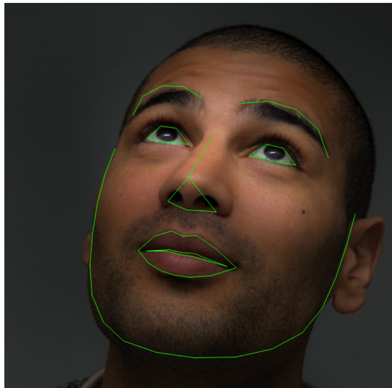
总之,每一张脸的68个不同的地标点(x,y)都会被注释出来
⚠️从here这里下载数据并将其放在目录 ‘data/faces/’下。这个数据集实际上是通过对一些标记为“face”的imagenet图像应用出色的dlib pose估计生成的。
来自csv文件的带有注释数据集将如下所示:
image_name,part_0_x,part_0_y,part_1_x,part_1_y,part_2_x,part_2_y,part_3_x,part_3_y,part_4_x,part_4_y,part_5_x,part_5_y,part_6_x,part_6_y,part_7_x,part_7_y,part_8_x,part_8_y,part_9_x,part_9_y,part_10_x,part_10_y,part_11_x,part_11_y,part_12_x,part_12_y,part_13_x,part_13_y,part_14_x,part_14_y,part_15_x,part_15_y,part_16_x,part_16_y,part_17_x,part_17_y,part_18_x,part_18_y,part_19_x,part_19_y,part_20_x,part_20_y,part_21_x,part_21_y,part_22_x,part_22_y,part_23_x,part_23_y,part_24_x,part_24_y,part_25_x,part_25_y,part_26_x,part_26_y,part_27_x,part_27_y,part_28_x,part_28_y,part_29_x,part_29_y,part_30_x,part_30_y,part_31_x,part_31_y,part_32_x,part_32_y,part_33_x,part_33_y,part_34_x,part_34_y,part_35_x,part_35_y,part_36_x,part_36_y,part_37_x,part_37_y,part_38_x,part_38_y,part_39_x,part_39_y,part_40_x,part_40_y,part_41_x,part_41_y,part_42_x,part_42_y,part_43_x,part_43_y,part_44_x,part_44_y,part_45_x,part_45_y,part_46_x,part_46_y,part_47_x,part_47_y,part_48_x,part_48_y,part_49_x,part_49_y,part_50_x,part_50_y,part_51_x,part_51_y,part_52_x,part_52_y,part_53_x,part_53_y,part_54_x,part_54_y,part_55_x,part_55_y,part_56_x,part_56_y,part_57_x,part_57_y,part_58_x,part_58_y,part_59_x,part_59_y,part_60_x,part_60_y,part_61_x,part_61_y,part_62_x,part_62_y,part_63_x,part_63_y,part_64_x,part_64_y,part_65_x,part_65_y,part_66_x,part_66_y,part_67_x,part_67_y
0805personali01.jpg,27,83,27,98,29,113,33,127,39,139,49,150,60,159,73,166,87,168,100,166,111,160,120,151,128,141,133,128,137,116,138,102,138,89,44,70,53,66,63,65,73,66,82,70,103,72,111,69,120,68,128,69,135,73,92,82,92,91,92,100,92,109,82,117,86,119,91,120,95,119,99,118,55,82,62,78,70,79,76,84,69,86,61,85,106,86,111,81,119,81,125,85,120,88,112,88,71,137,78,131,85,127,90,129,94,129,99,134,103,142,97,144,92,145,88,145,83,144,77,141,75,137,85,134,89,135,93,136,100,141,93,135,89,135,84,134
1084239450_e76e00b7e7.jpg,70,236,71,257,75,278,82,299,90,320,100,340,111,359,126,375,149,379,175,376,197,364,218,346,236,322,249,296,254,266,256,237,256,207,65,210,69,197,80,193,93,196,106,201,143,196,160,185,179,180,198,182,212,193,127,212,126,230,126,248,125,266,113,279,122,283,132,285,143,281,154,277,81,224,87,216,98,215,110,222,99,225,88,227,159,216,170,207,181,206,192,212,183,215,171,216,110,314,117,310,126,308,135,309,147,307,164,306,184,307,167,317,152,321,139,323,130,322,120,318,114,313,127,312,136,313,148,311,179,308,149,312,137,314,128,312
...
记录数据集中每张图片被标注的68个点
让我们快速读取CSV并获得一个(N, 2)数组中的注释,其中N是地标的数量,即第几个图片。
landmarks_frame = pd.read_csv('data/faces/face_landmarks.csv')

n = 65
img_name = landmarks_frame.iloc[n, 0] #得到图片的image_name信息
landmarks = landmarks_frame.iloc[n, 1:].as_matrix() #得到该图片的所有地标点信息
landmarks = landmarks.astype('float').reshape(-1, 2) #现降值转称类型float,.reshape函数用于将值变为一个列为2的矩阵,-1表示行根据情况自动判断,因为这里有68对(x,y),所以行为68

print('Image name: {}'.format(img_name)) #图像名
print('Landmarks shape: {}'.format(landmarks.shape)) #矩阵格式
print('First 4 Landmarks: {}'.format(landmarks[:4])) #得到前4个坐标点
返回:
Image name: person-7.jpg
Landmarks shape: (68, 2)
First 4 Landmarks: [[32. 65.]
 [33. 76.]
 [34. 86.]
 [34. 97.]]
然后写一个简单的帮助函数去显示一张图像和他的地标点,然后显示一个例子:
def show_landmarks(image, landmarks):
    """Show image with landmarks"""
    plt.imshow(image)
    #作用是在图上将坐标点标出来
    plt.scatter(landmarks[:, 0], landmarks[:, 1], s=10, marker='.', c='r') #参数为(x, y, s=点的大小,marker=标志点的形状,c=颜色)
    plt.pause(0.001)  # pause a bit so that plots are updated

plt.figure()
show_landmarks(io.imread(os.path.join('data/faces/', img_name)),landmarks)
plt.show()
显示:

Dataset class
torch.utils.data.Dataset是代表数据集的一个抽象类。你定制的数据集应该继承与Dataset并覆盖下面的方法:
__len__:这样调用len(dataset)函数才回返回数据集的大小- __getitem__:用来支持使用索引,如dataset[i]可以用来得到第i个例子
让我们为我们的面部地标数据集创建一个数据集类别。我们将会在__init__中读取csv,在__getitem__中读取图片。这是一种内存效率,因为所有的图片不是一次存储在内存中,而是根据需要读取。
我们数据集的例子将是字典格式:{'image': image, 'landmarks': landmarks}。我们数据集将会设置一个可选参数transform,这样任何需要做的处理将可以应用到例子当中。我们将会在下一部分看见transform的用处
class FaceLandmarksDataset(Dataset):
    """Face Landmarks dataset."""

    def __init__(self, csv_file, root_dir, transform=None):
        """
        Args:
            csv_file (string): 指明带有注释的csv文件的路径
            root_dir (string): 指明所有图片的文件夹
            transform (callable, optional): 指明应用在例子中的可选转换方式
        """
        self.landmarks_frame = pd.read_csv(csv_file)
        self.root_dir = root_dir
        self.transform = transform

    def __len__(self):
        return len(self.landmarks_frame)

    def __getitem__(self, idx):
        img_name = os.path.join(self.root_dir,self.landmarks_frame.iloc[idx, 0]) #得到图片名
        image = io.imread(img_name) #使用图片名去获得图片
        landmarks = self.landmarks_frame.iloc[idx, 1:].as_matrix() #然后得到她们的地标点,生成矩阵
        landmarks = landmarks.astype('float').reshape(-1, 2) #然后转换点类型为float,将矩阵转成68*2格式
        sample = {'image': image, 'landmarks': landmarks} #然后以字典的格式输出

        if self.transform: #对得到的例子进行transform
            sample = self.transform(sample)

        return sample
让我们实例化这个类并遍历数据示例。我们将打印前4个样品的大小并显示它们的地标。
face_dataset = FaceLandmarksDataset(csv_file='data/faces/face_landmarks.csv',root_dir='data/faces/')

fig = plt.figure()

for i in range(len(face_dataset)):
    sample = face_dataset[i]

    print(i, sample['image'].shape, sample['landmarks'].shape)

    ax = plt.subplot(1, 4, i + 1)
    plt.tight_layout()
    ax.set_title('Sample #{}'.format(i))
    ax.axis('off')
    show_landmarks(**sample)

    if i == 3:
        plt.show()
        break
显示:
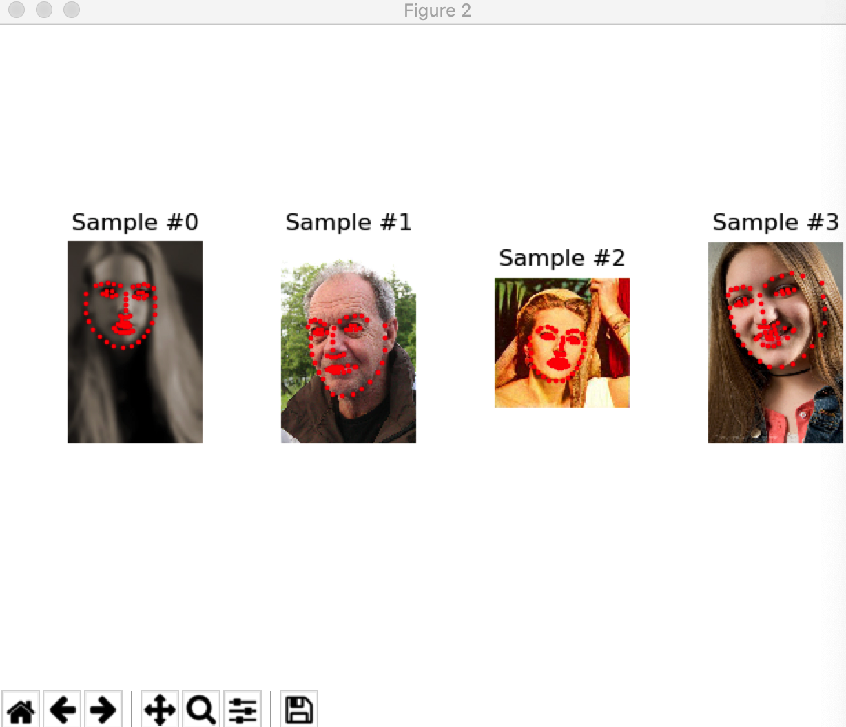
输出:
0 (324, 215, 3) (68, 2) #numpy表示为(height,width,channel)
1 (500, 333, 3) (68, 2)
2 (250, 258, 3) (68, 2)
3 (434, 290, 3) (68, 2)
Transforms
从上面我们可以看到的一个问题是样品的尺寸不一样。大多数神经网络期望图像的大小是固定的。因此,我们需要编写一些预处理代码。让我们创建三个转换:
- Rescale:对图像进行缩放
- RandomCrop:从图像中随机裁剪。这是用于进行数据扩充。
- ToTensor:要将numpy图像转换为torch图像(我们需要交换轴)。
我们将会将他们写成可调用的类,而不是简单的函数,这样transform的参数就不需要在每次调用的时候被传递了。为了这个,我们需要实现__call__方法,如果需要的话,还实现__init__方法。我们可以像这样使用transform:
tsfm = Transform(params) #调用__init__
transformed_sample = tsfm(sample) #调用__call__
观察下面transform是如何被使用到图像和地标上的:
class Rescale(object):
    """根据给定的大小在示例中所放图像

    Args:
        output_size (tuple or int): 期望的输出大小。如果是tuple,输出将与output_size相匹配。如果是int,较小的图像边缘匹配到output_size保持h/w比率不变。
    """

    def __init__(self, output_size): #output_size只能是int或tuple两种类型
        assert isinstance(output_size, (int, tuple))
        self.output_size = output_size

    def __call__(self, sample):
        image, landmarks = sample['image'], sample['landmarks']

        h, w = image.shape[:2] #得到图片的宽高
        if isinstance(self.output_size, int):#如果给的是int,则保证h/w比率不变
            if h > w:
                new_h, new_w = self.output_size * h / w, self.output_size
            else:
                new_h, new_w = self.output_size, self.output_size * w / h
        else: #如果给的是tuple,则是直接给了(height,width)
            new_h, new_w = self.output_size

        new_h, new_w = int(new_h), int(new_w)

        img = transform.resize(image, (new_h, new_w))

        # h and w are swapped for landmarks because for images,
        # x and y axes are axis 1 and 0 respectively
        landmarks = landmarks * [new_w / w, new_h / h]

        return {'image': img, 'landmarks': landmarks}


class RandomCrop(object):
    """随机裁剪示例中的图片.

    Args:
        output_size (tuple or int): 期望的输出大小。如果为int,则裁剪为正方形
    """

    def __init__(self, output_size):
        assert isinstance(output_size, (int, tuple))
        if isinstance(output_size, int):
            self.output_size = (output_size, output_size)
        else:
            assert len(output_size) == 2
            self.output_size = output_size

    def __call__(self, sample):
        image, landmarks = sample['image'], sample['landmarks']

        h, w = image.shape[:2]
        new_h, new_w = self.output_size

        top = np.random.randint(0, h - new_h)
        left = np.random.randint(0, w - new_w)

        image = image[top: top + new_h,
                      left: left + new_w]

        landmarks = landmarks - [left, top]

        return {'image': image, 'landmarks': landmarks}


class ToTensor(object):
    """Convert ndarrays in sample to Tensors."""

    def __call__(self, sample):
        image, landmarks = sample['image'], sample['landmarks']

        # swap color axis because
        # numpy image: H x W x C
        # torch image: C X H X W
        image = image.transpose((2, 0, 1))
        return {'image': torch.from_numpy(image),
                'landmarks': torch.from_numpy(landmarks)}
Compose transforms
现在,我们将transforms应用于一个示例。
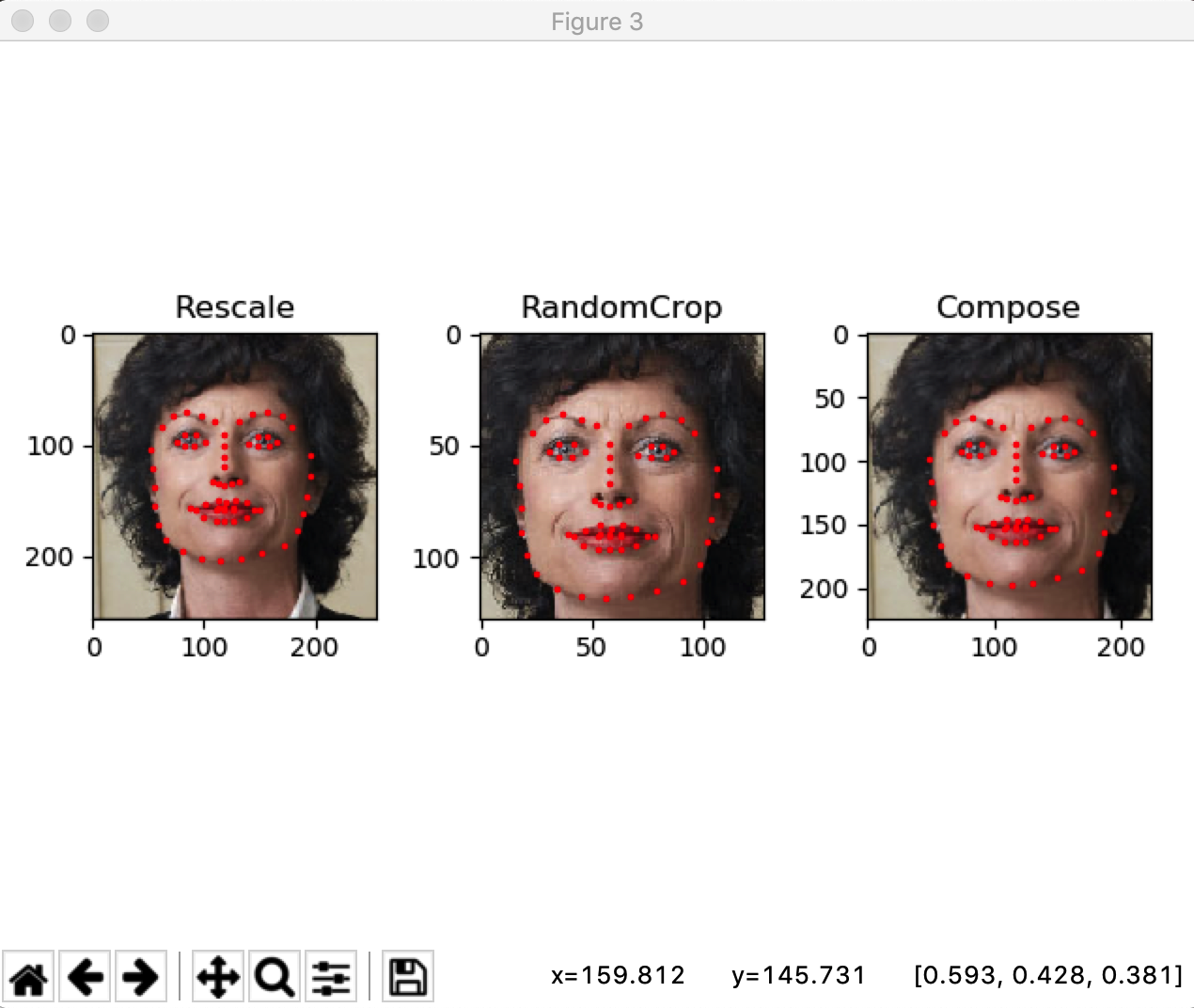
假设我们想把图像的短边重设为256然后随机裁剪一个224的正方形,即我们想组合Rescale和RandomCrop变换。torchvision.transforms.Compose是一个允许我们这样做的简单的可调用类。
scale = Rescale(256)
crop = RandomCrop(128)
composed = transforms.Compose([Rescale(256),
                               RandomCrop(224)])

# Apply each of the above transforms on sample.
fig = plt.figure()
sample = face_dataset[65]

#迭代进行三种转换
for i, tsfrm in enumerate([scale, crop, composed]):
    transformed_sample = tsfrm(sample)

    ax = plt.subplot(1, 3, i + 1)
    plt.tight_layout()
    ax.set_title(type(tsfrm).__name__)
    show_landmarks(**transformed_sample)

plt.show()
显示:
Iterating through the dataset
让我们把这些放在一起创建一个具有组合transforms的数据集。综上所述,每次采样该数据集时:
- 从文件中动态读取图像
- transforms应用于读取的图像
- 由于其中一种转换是随机的,因此数据在抽样时得到了扩充
如之前一样使用for i in range循环去迭代创建的数据集:
transformed_dataset = FaceLandmarksDataset(csv_file='data/faces/face_landmarks.csv',
                                           root_dir='data/faces/',
                                           transform=transforms.Compose([
                                               Rescale(256),
                                               RandomCrop(224),
                                               ToTensor()
                                           ]))

for i in range(len(transformed_dataset)):
    sample = transformed_dataset[i]

    print(i, sample['image'].size(), sample['landmarks'].size())

    if i == 3: #仅输出四张图片
        break
返回:
0 torch.Size([3, 224, 224]) torch.Size([68, 2]) #tensor表示为(channel,height,width)
1 torch.Size([3, 224, 224]) torch.Size([68, 2])
2 torch.Size([3, 224, 224]) torch.Size([68, 2])
3 torch.Size([3, 224, 224]) torch.Size([68, 2])
然而,由于使用简单的for循环遍历数据,我们正在丢失很多特性。特别是,我们正在错过:
- 批处理数据
- 移动数据
- 使用多处理工作者并行加载数据。
torch.utils.data.DataLoader 是提供所有这些特性的一个迭代器。下面使用的参数应该是清楚的。一个令人感兴趣的参数是collate_fn。你可以使用collate_fn指定需要如何对样本进行批处理。然而,默认的排序对于大多数用例来说应该是有效的。
dataloader = DataLoader(transformed_dataset, batch_size=4, #对数据进行批处理,4张图片为一批,然后将数据集进行打乱,并行获取照片的进程为4
                        shuffle=True, num_workers=4)


# Helper function to show a batch
def show_landmarks_batch(sample_batched):
    """Show image with landmarks for a batch of samples."""
    images_batch, landmarks_batch = \
            sample_batched['image'], sample_batched['landmarks']
    batch_size = len(images_batch)
    im_size = images_batch.size(2)

    grid = utils.make_grid(images_batch)
    plt.imshow(grid.numpy().transpose((1, 2, 0)))

    for i in range(batch_size):
        plt.scatter(landmarks_batch[i, :, 0].numpy() + i * im_size,
                    landmarks_batch[i, :, 1].numpy(),
                    s=10, marker='.', c='r')

        plt.title('Batch from dataloader')

for i_batch, sample_batched in enumerate(dataloader):
    print(i_batch, sample_batched['image'].size(),
          sample_batched['landmarks'].size())

    # 观察4批数据就停止
    if i_batch == 3:
        plt.figure()
        show_landmarks_batch(sample_batched) #将图显示出来,仅显示第四批图
        plt.axis('off')
        plt.ioff()
        plt.show()
        break
显示:
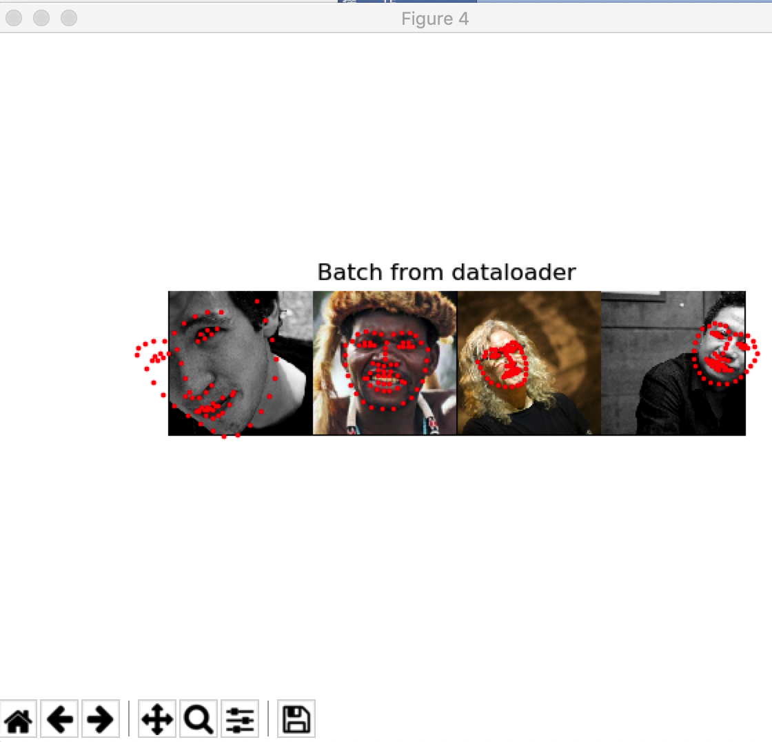
返回:
0 torch.Size([4, 3, 224, 224]) torch.Size([4, 68, 2])
1 torch.Size([4, 3, 224, 224]) torch.Size([4, 68, 2])
2 torch.Size([4, 3, 224, 224]) torch.Size([4, 68, 2])
3 torch.Size([4, 3, 224, 224]) torch.Size([4, 68, 2])
Afterword: torchvision
在本教程中,我们已经了解了如何编写和使用数据集、转换和dataloader。torchvision包提供了一些常见的数据集和转换。你甚至可能不需要编写自定义类。在torchvision中可用的一个更通用的数据集是ImageFolder。它假设图像的组织方式如下:
root/ants/xxx.png
root/ants/xxy.jpeg
root/ants/xxz.png
.
.
.
root/bees/123.jpg
root/bees/nsdf3.png
root/bees/asd932_.png
其中 ‘ants’, ‘bees’等是类标签。在PIL.Image上操作的类似的通用转换,如RandomHorizontalFlip, Scale,也是可用的。你可以使用这些来编写这样一个dataloader:
#所以上面的一堆很复杂的数据梳理其实都可以写成下面这种十分简单的格式
import torch
from torchvision import transforms, datasets

#声明要对数据进行的transforms操作
data_transform = transforms.Compose([
        transforms.RandomSizedCrop(224),
        transforms.RandomHorizontalFlip(),
        transforms.ToTensor(),
        transforms.Normalize(mean=[0.485, 0.456, 0.406],
                             std=[0.229, 0.224, 0.225])
    ])
#然后将这些transforms操作应用到数据集中
hymenoptera_dataset = datasets.ImageFolder(root='hymenoptera_data/train',
                                           transform=data_transform)
#然后将她们进行批处理等操作
dataset_loader = torch.utils.data.DataLoader(hymenoptera_dataset,
                                             batch_size=4, shuffle=True,
                                             num_workers=4)