吴恩达机器学习课程笔记+代码实现(13)Python实现神经网络中的反向传播(Programming Exercise 4)

Programming Exercise 4:NN back propagation

Python版本3.6
编译环境：anaconda Jupyter Notebook
链接：实验数据和实验指导书
提取码：i7co
本章课程笔记部分见：神经网络：表述(Neural Networks: Representation) 神经网络的学习(Neural Networks: Learning)

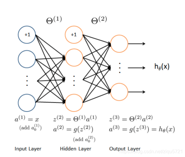
本次练习中，我们将再次处理手写数字数据集，这次使用反向传播的前馈神经网络,通过反向传播算法实现神经网络成本函数和梯度计算的非正则化和正则化版本。 我们还将实现随机权重初始化和使用网络进行预测的方法。

%matplotlib inline
#IPython的内置magic函数，可以省掉plt.show()，在其他IDE中是不会支持的
import numpy as np
import pandas as pd
import matplotlib as mpl
import matplotlib.pyplot as plt
import seaborn as sns
sns.set(style="whitegrid",color_codes=True)
import scipy.io as sio
import scipy.optimize as opt
from sklearn.metrics import classification_report#这个包是评价报告

加载数据集和可视化

同exercise3

data = sio.loadmat('ex4data1.mat')
data

{'__header__': b'MATLAB 5.0 MAT-file, Platform: GLNXA64, Created on: Sun Oct 16 13:09:09 2011',
 '__version__': '1.0',
 '__globals__': [],
 'X': array([[0., 0., 0., ..., 0., 0., 0.],
        [0., 0., 0., ..., 0., 0., 0.],
        [0., 0., 0., ..., 0., 0., 0.],
        ...,
        [0., 0., 0., ..., 0., 0., 0.],
        [0., 0., 0., ..., 0., 0., 0.],
        [0., 0., 0., ..., 0., 0., 0.]]),
 'y': array([[10],
        [10],
        [10],
        ...,
        [ 9],
        [ 9],
        [ 9]], dtype=uint8)}

X = data.get('X')
y = data.get('y')
y = y.reshape(y.shape[0])
print(X.shape,y.shape)

(5000, 400) (5000,)

def plot_100_image(X):
    """ sample 100 image and show them
    assume the image is square

    X : (5000, 400)
    """
    size = int(np.sqrt(X.shape[1]))

    # sample 100 image, reshape, reorg it
    sample_idx = np.random.choice(np.arange(X.shape[0]), 100)  # 100*400
    sample_images = X[sample_idx, :]

    fig, ax_array = plt.subplots(nrows=10, ncols=10, sharey=True, sharex=True, figsize=(8, 8))

    for r in range(10):
        for c in range(10):
            ax_array[r, c].matshow(sample_images[10 * r + c].reshape((size, size)),
                                   cmap=mpl.cm.binary)
            plt.xticks(np.array([]))
            plt.yticks(np.array([]))

plot_100_image(X)

数据预处理

X = np.insert(X, 0, np.ones(X.shape[0]), axis=1)#增加全部为1的一列
X.shape

(5000, 401)

def expand_y(y):
#     """expand 5000*1 into 5000*10
#     where y=10 -> [0, 0, 0, 0, 0, 0, 0, 0, 0, 1]: ndarray
#     """
    res = []
    for i in y:
        y_array = np.zeros(10)
        y_array[i - 1] = 1

        res.append(y_array)

    return np.array(res)
# from sklearn.preprocessing import OneHotEncoder
# encoder = OneHotEncoder(sparse=False)
# y_onehot = encoder.fit_transform(y)
# y_onehot.shape #这个函数与expand_y(y)一致

y = expand_y(y)
y

array([[0., 0., 0., ..., 0., 0., 1.],
       [0., 0., 0., ..., 0., 0., 1.],
       [0., 0., 0., ..., 0., 0., 1.],
       ...,
       [0., 0., 0., ..., 0., 1., 0.],
       [0., 0., 0., ..., 0., 1., 0.],
       [0., 0., 0., ..., 0., 1., 0.]])

读取权重

def load_weight(path):
    data = sio.loadmat(path)
    return data['Theta1'], data['Theta2']

t1, t2 = load_weight('ex4weights.mat')
t1.shape, t2.shape

((25, 401), (10, 26))

def serialize(a, b):
  
    return np.concatenate((np.ravel(a), np.ravel(b)))
# 序列化2矩阵
# 在这个nn架构中，我们有theta1（25,401），theta2（10,26），它们的梯度是delta1，delta2  

theta = serialize(t1, t2)  # 扁平化参数，25*401+10*26=10285
theta.shape

(10285,)

feed forward（前向传播）

(400 + 1) -> (25 + 1) -> (10)

def deserialize(seq):
#     """into ndarray of (25, 401), (10, 26)"""
    return seq[:25 * 401].reshape(25, 401), seq[25 * 401:].reshape(10, 26)

def feed_forward(theta, X):
    """apply to architecture 400+1 * 25+1 *10
    X: 5000 * 401
    """

    t1, t2 = deserialize(theta)  # t1: (25,401) t2: (10,26)
    m = X.shape[0]
    a1 = X  # 5000 * 401

    z2 = a1 @ t1.T  # 5000 * 25
    a2 = np.insert(sigmoid(z2), 0, np.ones(m), axis=1)  # 5000*26

    z3 = a2 @ t2.T  # 5000 * 10
    h = sigmoid(z3)  # 5000*10, this is h_theta(X)

    return a1, z2, a2, z3, h  # you need all those for backprop

def sigmoid(z):
    return 1 / (1 + np.exp(-z))

_, _, _, _, h = feed_forward(theta, X)
h # 5000*10

array([[1.12661530e-04, 1.74127856e-03, 2.52696959e-03, ...,
        4.01468105e-04, 6.48072305e-03, 9.95734012e-01],
       [4.79026796e-04, 2.41495958e-03, 3.44755685e-03, ...,
        2.39107046e-03, 1.97025086e-03, 9.95696931e-01],
       [8.85702310e-05, 3.24266731e-03, 2.55419797e-02, ...,
        6.22892325e-02, 5.49803551e-03, 9.28008397e-01],
       ...,
       [5.17641791e-02, 3.81715020e-03, 2.96297510e-02, ...,
        2.15667361e-03, 6.49826950e-01, 2.42384687e-05],
       [8.30631310e-04, 6.22003774e-04, 3.14518512e-04, ...,
        1.19366192e-02, 9.71410499e-01, 2.06173648e-04],
       [4.81465717e-05, 4.58821829e-04, 2.15146201e-05, ...,
        5.73434571e-03, 6.96288990e-01, 8.18576980e-02]])

代价函数

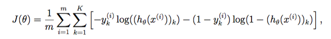
def cost(theta, X, y):
#     """calculate cost
#     y: (m, k) ndarray
#     """
    m = X.shape[0]  # get the data size m

    _, _, _, _, h = feed_forward(theta, X)

    # np.multiply is pairwise operation
    pair_computation = -np.multiply(y, np.log(h)) - np.multiply((1 - y), np.log(1 - h))

    return pair_computation.sum() / m

cost(theta, X, y)

0.2876291651613189

正则化代价函数

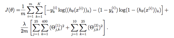
def regularized_cost(theta, X, y, l=1):
    """the first column of t1 and t2 is intercept theta, ignore them when you do regularization"""
    t1, t2 = deserialize(theta)  # t1: (25,401) t2: (10,26)
    m = X.shape[0]

    reg_t1 = (l / (2 * m)) * np.power(t1[:, 1:], 2).sum()  # this is how you ignore first col
    reg_t2 = (l / (2 * m)) * np.power(t2[:, 1:], 2).sum()

    return cost(theta, X, y) + reg_t1 + reg_t2

regularized_cost(theta, X, y)

0.38376985909092365

反向传播

读取数据和权重过程与前向传播相同

X.shape,y.shape

((5000, 401), (5000, 10))

t1.shape, t2.shape

((25, 401), (10, 26))

theta.shape

(10285,)

def sigmoid_gradient(z):
    """
    pairwise op is key for this to work on both vector and matrix
    """
    return np.multiply(sigmoid(z), 1 - sigmoid(z))

sigmoid_gradient(0)

0.25

theta gradient

super hard to get this right… the dimension is so confusing

def gradient(theta, X, y):
    # initialize
    t1, t2 = deserialize(theta)  # t1: (25,401) t2: (10,26)
    m = X.shape[0]

    delta1 = np.zeros(t1.shape)  # (25, 401)
    delta2 = np.zeros(t2.shape)  # (10, 26)

    a1, z2, a2, z3, h = feed_forward(theta, X)

    for i in range(m):
        a1i = a1[i, :]  # (1, 401)
        z2i = z2[i, :]  # (1, 25)
        a2i = a2[i, :]  # (1, 26)

        hi = h[i, :]    # (1, 10)
        yi = y[i, :]    # (1, 10)

        d3i = hi - yi  # (1, 10)

        z2i = np.insert(z2i, 0, np.ones(1))  # make it (1, 26) to compute d2i
        d2i = np.multiply(t2.T @ d3i, sigmoid_gradient(z2i))  # (1, 26)

        # careful with np vector transpose
        delta2 += np.matrix(d3i).T @ np.matrix(a2i)  # (1, 10).T @ (1, 26) -> (10, 26)
        delta1 += np.matrix(d2i[1:]).T @ np.matrix(a1i)  # (1, 25).T @ (1, 401) -> (25, 401)

    delta1 = delta1 / m
    delta2 = delta2 / m

    return serialize(delta1, delta2)

d1, d2 = deserialize(gradient(theta, X, y))

d1.shape, d2.shape

((25, 401), (10, 26))

梯度校验

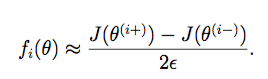
def gradient_checking(theta, X, y, epsilon, regularized=False):
    def a_numeric_grad(plus, minus, regularized=False):
        """calculate a partial gradient with respect to 1 theta"""
        if regularized:
            return (regularized_cost(plus, X, y) - regularized_cost(minus, X, y)) / (epsilon * 2)
        else:
            return (cost(plus, X, y) - cost(minus, X, y)) / (epsilon * 2)

    theta_matrix = expand_array(theta)  # expand to (10285, 10285)
    epsilon_matrix = np.identity(len(theta)) * epsilon

    plus_matrix = theta_matrix + epsilon_matrix
    minus_matrix = theta_matrix - epsilon_matrix

    # calculate numerical gradient with respect to all theta
    numeric_grad = np.array([a_numeric_grad(plus_matrix[i], minus_matrix[i], regularized)
                                    for i in range(len(theta))])

    # analytical grad will depend on if you want it to be regularized or not
    analytic_grad = regularized_gradient(theta, X, y) if regularized else gradient(theta, X, y)

    # If you have a correct implementation, and assuming you used EPSILON = 0.0001
    # the diff below should be less than 1e-9
    # this is how original matlab code do gradient checking
    diff = np.linalg.norm(numeric_grad - analytic_grad) / np.linalg.norm(numeric_grad + analytic_grad)

    print('If your backpropagation implementation is correct,\nthe relative difference will be smaller than 10e-9 (assume epsilon=0.0001).\nRelative Difference: {}\n'.format(diff))

def expand_array(arr):
    """replicate array into matrix
    [1, 2, 3]

    [[1, 2, 3],
     [1, 2, 3],
     [1, 2, 3]]
    """
    # turn matrix back to ndarray
    return np.array(np.matrix(np.ones(arr.shape[0])).T @ np.matrix(arr))

gradient_checking(theta, X, y, epsilon= 0.01)#这个运行很慢，谨慎运行

If your backpropagation implementation is correct,
the relative difference will be smaller than 10e-9 (assume epsilon=0.0001).
Relative Difference: 2.0654715779819265e-05

regularized gradient

Use normal gradient + regularized term

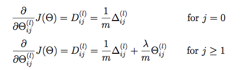
def regularized_gradient(theta, X, y, l=1):
    """don't regularize theta of bias terms"""
    m = X.shape[0]
    delta1, delta2 = deserialize(gradient(theta, X, y))
    t1, t2 = deserialize(theta)

    t1[:, 0] = 0
    reg_term_d1 = (l / m) * t1
    delta1 = delta1 + reg_term_d1

    t2[:, 0] = 0
    reg_term_d2 = (l / m) * t2
    delta2 = delta2 + reg_term_d2

    return serialize(delta1, delta2)

gradient_checking(theta, X, y, epsilon=0.01, regularized=True)

If your backpropagation implementation is correct,
the relative difference will be smaller than 10e-9 (assume epsilon=0.0001).
Relative Difference: 3.028117929073821e-05

train the model

remember to randomly initlized the parameters to break symmetry

take a look at the doc of this argument: jac

jac : bool or callable, optional
Jacobian (gradient) of objective function. Only for CG, BFGS, Newton-CG, L-BFGS-B, TNC, SLSQP, dogleg, trust-ncg. If jac is a Boolean and is True, fun is assumed to return the gradient along with the objective function. If False, the gradient will be estimated numerically. jac can also be a callable returning the gradient of the objective. In this case, it must accept the same arguments as fun.

it means if your backprop function return (cost, grad), you could set jac=True

This is the implementation of http://nbviewer.jupyter.org/github/jdwittenauer/ipython-notebooks/blob/master/notebooks/ml/ML-Exercise4.ipynb

but I choose to seperate them

def random_init(size):
    return np.random.uniform(-0.12, 0.12, size)

def nn_training(X, y):
    """regularized version
    the architecture is hard coded here... won't generalize
    """
    init_theta = random_init(10285)  # 25*401 + 10*26

    res = opt.minimize(fun=regularized_cost,
                       x0=init_theta,
                       args=(X, y, 1),
                       method='TNC',
                       jac=regularized_gradient,
                       options={'maxiter': 400})
    return res

res = nn_training(X, y)
res

     fun: 0.38511397411332776
     jac: array([ 1.55865287e-04, -6.22780032e-06,  9.32353468e-06, ...,
        1.22243669e-05, -1.28445537e-04, -3.77201590e-05])
 message: 'Linear search failed'
    nfev: 238
     nit: 15
  status: 4
 success: False
       x: array([ 0.        , -0.031139  ,  0.04661767, ..., -3.38149892,
        2.04519846, -4.71640687])

准确率

y = data.get('y')
y = y.reshape(y.shape[0])  # make it back to column vector

y[:20]

array([10, 10, 10, 10, 10, 10, 10, 10, 10, 10, 10, 10, 10, 10, 10, 10, 10,
       10, 10, 10], dtype=uint8)

final_theta = res.x

def show_accuracy(theta, X, y):
    _, _, _, _, h = feed_forward(theta, X)

    y_pred = np.argmax(h, axis=1) + 1

    print(classification_report(y, y_pred))

show_accuracy(final_theta,X,y)

              precision    recall  f1-score   support

           1       0.98      0.98      0.98       500
           2       0.97      0.97      0.97       500
           3       0.90      0.98      0.94       500
           4       1.00      0.91      0.95       500
           5       1.00      0.82      0.90       500
           6       0.98      0.98      0.98       500
           7       0.99      0.94      0.97       500
           8       0.87      0.99      0.93       500
           9       0.93      0.96      0.95       500
          10       0.95      1.00      0.97       500

   micro avg       0.95      0.95      0.95      5000
   macro avg       0.96      0.95      0.95      5000
weighted avg       0.96      0.95      0.95      5000

显示隐藏层

def plot_hidden_layer(theta):
    """
    theta: (10285, )
    """
    final_theta1, _ = deserialize(theta)
    hidden_layer = final_theta1[:, 1:]  # ger rid of bias term theta

    fig, ax_array = plt.subplots(nrows=5, ncols=5, sharey=True, sharex=True, figsize=(5, 5))

    for r in range(5):
        for c in range(5):
            ax_array[r, c].matshow(hidden_layer[5 * r + c].reshape((20, 20)),
                                   cmap=mpl.cm.binary)
            plt.xticks(np.array([]))
            plt.yticks(np.array([]))


# nn functions starts here ---------------------------
# ps. all the y here is expanded version (5000,10)

plot_hidden_layer(final_theta)