代码:
%% ++++++++++++++++++++++++++++++++++++++++++++++++++++++++++++++++++++++++++++++++
%% Output Info about this m-file
fprintf('\n***********************************************************\n');
fprintf(' <DSP using MATLAB> Problem 7.9 \n\n');
banner();
%% ++++++++++++++++++++++++++++++++++++++++++++++++++++++++++++++++++++++++++++++++
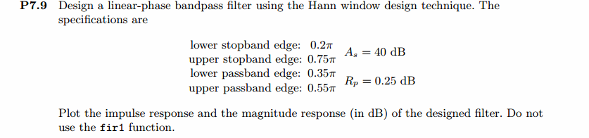
ws1 = 0.2*pi; wp1 = 0.35*pi; wp2 = 0.55*pi; ws2 = 0.75*pi; As = 40;
tr_width = min((wp1-ws1), (ws2-wp2));
M = ceil(6.2*pi/tr_width) + 1; % Hann Window
fprintf('\nFilter Length is %d.\n', M);
n = [0:1:M-1]; wc1 = (ws1+wp1)/2; wc2 = (wp2+ws2)/2;
%wc = (ws + wp)/2, % ideal LPF cutoff frequency
hd = ideal_lp(wc2, M) - ideal_lp(wc1, M);
w_han = (hann(M))'; h = hd .* w_han;
[db, mag, pha, grd, w] = freqz_m(h, [1]); delta_w = 2*pi/1000;
[Hr,ww,P,L] = ampl_res(h);
Rp = -(min(db(wp1/delta_w+1 : 1 : wp2/delta_w))); % Actual Passband Ripple
fprintf('\nActual Passband Ripple is %.4f dB.\n', Rp);
As = -round(max(db(ws2/delta_w+1 : 1 : 501))); % Min Stopband attenuation
fprintf('\nMin Stopband attenuation is %.4f dB.\n', As);
[delta1, delta2] = db2delta(Rp, As)
%Plot
figure('NumberTitle', 'off', 'Name', 'Problem 7.9 ideal_lp Method')
set(gcf,'Color','white');
subplot(2,2,1); stem(n, hd); axis([0 M-1 -0.4 0.5]); grid on;
xlabel('n'); ylabel('hd(n)'); title('Ideal Impulse Response');
subplot(2,2,2); stem(n, w_han); axis([0 M-1 0 1.1]); grid on;
xlabel('n'); ylabel('w(n)'); title('Hanning Window');
subplot(2,2,3); stem(n, h); axis([0 M-1 -0.4 0.5]); grid on;
xlabel('n'); ylabel('h(n)'); title('Actual Impulse Response');
subplot(2,2,4); plot(w/pi, db); axis([0 1 -150 10]); grid on;
set(gca,'YTickMode','manual','YTick',[-90,-45,0]);
set(gca,'YTickLabelMode','manual','YTickLabel',['90';'45';' 0']);
set(gca,'XTickMode','manual','XTick',[0,0.2,0.35,0.55,0.75,1]);
xlabel('frequency in \pi units'); ylabel('Decibels'); title('Magnitude Response in dB');
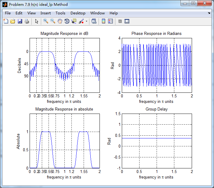
figure('NumberTitle', 'off', 'Name', 'Problem 7.9 h(n) ideal_lp Method')
set(gcf,'Color','white');
subplot(2,2,1); plot(w/pi, db); grid on; %axis([0 1 -100 10]);
xlabel('frequency in \pi units'); ylabel('Decibels'); title('Magnitude Response in dB');
set(gca,'YTickMode','manual','YTick',[-90,-45,0])
set(gca,'YTickLabelMode','manual','YTickLabel',['90';'45';' 0']);
set(gca,'XTickMode','manual','XTick',[0,0.2,0.35,0.55,0.75,1,1.2,1.55,2]);
subplot(2,2,3); plot(w/pi, mag); grid on; %axis([0 1 -100 10]);
xlabel('frequency in \pi units'); ylabel('Absolute'); title('Magnitude Response in absolute');
set(gca,'XTickMode','manual','XTick',[0,0.2,0.35,0.55,0.75,1,1.2,1.55,2]);
set(gca,'YTickMode','manual','YTick',[0.0,0.5,1.0])
subplot(2,2,2); plot(w/pi, pha); grid on; %axis([0 1 -100 10]);
xlabel('frequency in \pi units'); ylabel('Rad'); title('Phase Response in Radians');
subplot(2,2,4); plot(w/pi, grd*pi/180); grid on; %axis([0 1 -100 10]);
xlabel('frequency in \pi units'); ylabel('Rad'); title('Group Delay');
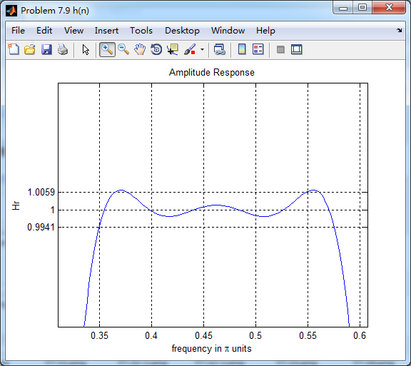
figure('NumberTitle', 'off', 'Name', 'Problem 7.9 h(n)')
set(gcf,'Color','white');
plot(ww/pi, Hr); grid on; %axis([0 1 -100 10]);
xlabel('frequency in \pi units'); ylabel('Hr'); title('Amplitude Response');
set(gca,'YTickMode','manual','YTick',[-delta2,0,delta2,1 - delta1,1, 1 + delta1])
%set(gca,'YTickLabelMode','manual','YTickLabel',['90';'45';' 0']);
%set(gca,'XTickMode','manual','XTick',[0,0.2,0.35,0.55,0.75,1,1.2,1.55,2]);
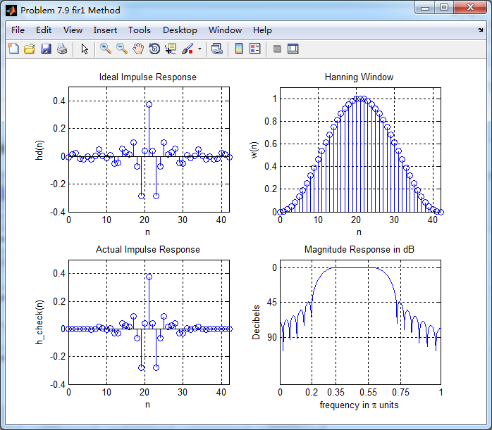
h_check = fir1(M-1, [wc1 wc2]/pi, 'bandpass', window(@hann,M));
[db, mag, pha, grd, w] = freqz_m(h_check, [1]);
[Hr,ww,P,L] = ampl_res(h_check);
figure('NumberTitle', 'off', 'Name', 'Problem 7.9 fir1 Method')
set(gcf,'Color','white');
subplot(2,2,1); stem(n, hd); axis([0 M-1 -0.4 0.5]); grid on;
xlabel('n'); ylabel('hd(n)'); title('Ideal Impulse Response');
subplot(2,2,2); stem(n, w_han); axis([0 M-1 0 1.1]); grid on;
xlabel('n'); ylabel('w(n)'); title('Hanning Window');
subplot(2,2,3); stem(n, h_check); axis([0 M-1 -0.4 0.5]); grid on;
xlabel('n'); ylabel('h\_check(n)'); title('Actual Impulse Response');
subplot(2,2,4); plot(w/pi, db); axis([0 1 -150 10]); grid on;
set(gca,'YTickMode','manual','YTick',[-90,-45,0])
set(gca,'YTickLabelMode','manual','YTickLabel',['90';'45';' 0']);
set(gca,'XTickMode','manual','XTick',[0,0.2,0.35,0.55,0.75,1]);
xlabel('frequency in \pi units'); ylabel('Decibels'); title('Magnitude Response in dB');
figure('NumberTitle', 'off', 'Name', 'Problem 7.9 h(n) fir1 Method')
set(gcf,'Color','white');
subplot(2,2,1); plot(w/pi, db); grid on; %axis([0 1 -100 10]);
xlabel('frequency in \pi units'); ylabel('Decibels'); title('Magnitude Response in dB');
set(gca,'YTickMode','manual','YTick',[-90,-45,0])
set(gca,'YTickLabelMode','manual','YTickLabel',['90';'45';' 0']);
set(gca,'XTickMode','manual','XTick',[0,0.2,0.35,0.55,0.75,1,1.2,1.55,2]);
subplot(2,2,3); plot(w/pi, mag); grid on; %axis([0 1 -100 10]);
xlabel('frequency in \pi units'); ylabel('Absolute'); title('Magnitude Response in absolute');
set(gca,'XTickMode','manual','XTick',[0,0.2,0.35,0.55,0.75,1,1.2,1.55,2]);
set(gca,'YTickMode','manual','YTick',[0.0,0.5,1.0])
subplot(2,2,2); plot(w/pi, pha); grid on; %axis([0 1 -100 10]);
xlabel('frequency in \pi units'); ylabel('Rad'); title('Phase Response in Radians');
subplot(2,2,4); plot(w/pi, grd*pi/180); grid on; %axis([0 1 -100 10]);
xlabel('frequency in \pi units'); ylabel('Rad'); title('Group Delay');
运行结果:
45dB满足设计要求。
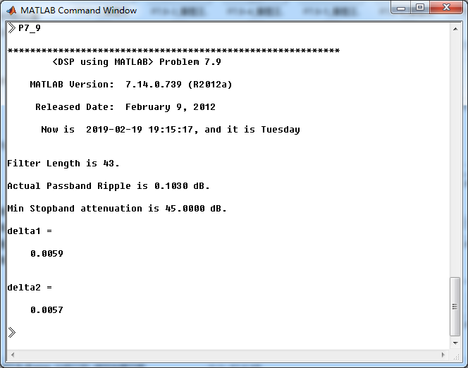
理想低通方法加窗截断,获得脉冲响应。其幅度响应(dB和Absolute单位)、相位响应、群延迟
振幅响应,通带部分(放大图)
振幅响应,阻带部分(放大图)

使用fir1函数获得脉冲响应,其幅度响应(dB和Absolute单位)、相位响应、群延迟响应