常见的数据类型:
- 一维: Series
- 二维: DataFrame
- 三维: Panel …
- 四维: Panel4D …
- N维: PanelND …
1. 创建DataFrame数据类型
DataFRame对象里面包含两个索引, 行索引(0轴, axis=0), 列索引(1轴, axis=1)
方法1: 通过列表创建
import pandas as pd
import numpy as np
li = [
[1, 2, 3, 4],
[2, 3, 4, 5]
]
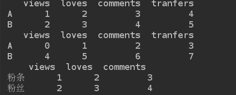
d1 = pd.DataFrame(data=li, index=['A', 'B'], columns=['views', 'loves', 'comments', 'tranfers'])
print(d1)
方法2: 通过numpy对象创建
narr = np.arange(8).reshape(2, 4)
d2 = pd.DataFrame(data=narr, index=['A', 'B'], columns=['views', 'loves', 'comments', 'tranfers'])
print(d2)
方法三: 通过字典的方式创建
dict = {
    'views': [1, 2, ],
    'loves': [2, 3, ],
    'comments': [3, 4, ]

}
d3 = pd.DataFrame(data=dict, index=['粉条', "粉丝"])
print(d3)
2. 日期操作
dates = pd.date_range(start='1/1/2018', end='1/08/2018')
print(dates)

# 行索引
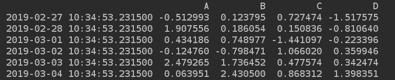
dates = pd.date_range(start='today', periods=6)#6天
# 数据
data_arr = np.random.randn(6, 4)
# 列索引
columns = ['A', 'B', 'C', 'D']
d4 = pd.DataFrame(data_arr, index=dates, columns=columns)
print(d4)
一维对象: 建立一个以2019年每一天作为索引, 值为随机数;
dates = pd.date_range(start='1/1/2019', end='12/31/2019', freq='D')
datas = np.random.randn(len(dates))
s1 = pd.Series(datas, index=dates)
print(s1[:10])
3. DataFrame的基本操作
1). 查看基础属性
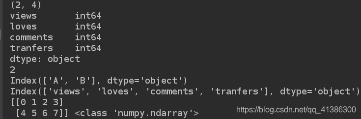
narr = np.arange(8).reshape(2, 4)
d2 = pd.DataFrame(data=narr, index=['A', 'B'], columns=['views', 'loves', 'comments', 'tranfers'])

print(d2.shape)  # 获取行数和列数;
print(d2.dtypes)  # 列数据类型
print(d2.ndim)  # 获取数据的维度
print(d2.index) # 行索引
print(d2.columns) # 列索引
print(d2.values, type(d2.values))   # 对象的值, 二维ndarray数组;
2). 数据整体状况的查询
显示头几行, 默认5行
print(d2.head(1))
显示倒数几行, 默认5行
print(d2.tail(1))
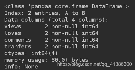
相关信息的预览: 行数, 列数, 列类型, 内存占用
print("info:", d2.info())
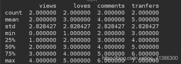
快速综合统计结果: 计数, 均值, 标准差, 最小值, 1/4位数, 中位数, 3/4位数, 最大值;
print(d2.describe())
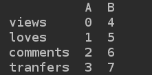
3). 转置操作
print(d2.T)
4). 按列进行排序
排序结果好像是根据第一列决定的
print(d2.sort_values(by="views", ascending=False))
5). 切片及查询
可以实现切片, 但是不能索引
print(d2[:1])
通过标签查询, 获取单列信息
print(d2['views'])
print('2:\n', d2.views)# 和上面是等价的;
通过标签查询多列信息
print(d2[['views', 'comments']])
6). 通过类似索引的方式查询;
- iloc(通过位置进行行数据的获取),
- loc(t通过标签索引行数据)
print(d2.iloc[0])

print(d2.iloc[-1:])

print(d2.loc['A'])

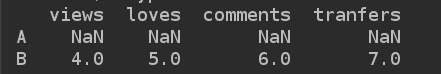
7). 更改pandas的值
d2.loc['A'] = np.nan
print(d2)
4. 从文件中读写数据
import pandas as pd
# 1). csv文件的写入
df = pd.DataFrame(
{'province': ['陕西', '陕西', '四川', '四川', '陕西'],
'city': ['咸阳', '宝鸡', '成都', '成都', '宝鸡'],
'count1': [1, 2, 3, 4, 5],
'count2': [1, 2, 33, 4, 5]
}
)
df.to_csv('doc/csvFile.csv')
print("csv文件保存成功")
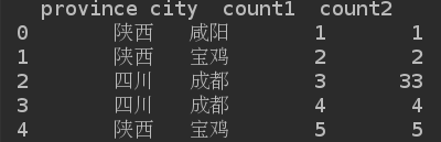
# 2). csv文件的读取
df2 = pd.read_csv('doc/csvFile.csv')
print(df2)
# 3). excel文件的写入
df2.to_excel("/tmp/excelFile.xlsx", sheet_name="省份统计")
print("excel文件保存成功")
5. 分组与聚合操作之groupby
pandas提供了一个灵活高效的groupby功能,
1). 它使你能以一种自然的方式对数据集进行切片、切块、摘要等操作。
2). 根据一个或多个键(可以是函数、数组或DataFrame列>名)拆分pandas对象。
3). 计算分组摘要统计,如计数、平均值、标准差,或用户自定义函数。
import pandas as pd
df = pd.DataFrame(
{'province': ['陕西', '陕西', '四川', '四川', '陕西'],
'city': ['咸阳', '宝鸡', '成都', '成都', '宝鸡'],
'count1': [1, 2, 3, 4, 5],
'count2': [1, 2, 33, 4, 5]
}
)
print(df)
# 根据某一列的key值进行统计分析;
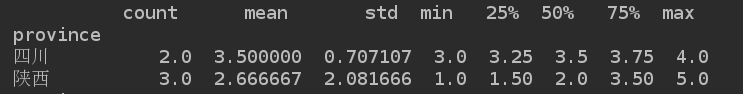
grouped = df['count1'].groupby(df['province'])
print(grouped.describe())
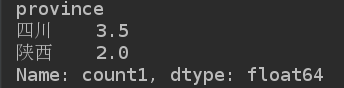
print(grouped.median())
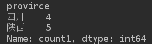
print(grouped.max())
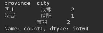
指定多个key值进行分类聚合
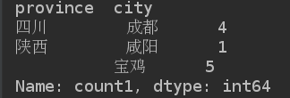
grouped = df['count1'].groupby([df['province'], df['city']])
print(grouped)
print(grouped.max())
print(grouped.sum())

print(grouped.count())
通过unstack方法, 实现层次化的索引
print(grouped.max().unstack())

案例
分析文件中的数据
文件:
,order_id,quantity,item_name,choice_description,item_price
0,1,1,Chips and Fresh Tomato Salsa,,$2.39
1,1,1,Izze,[Clementine],$3.39
2,1,1,Nantucket Nectar,[Apple],$3.39
3,1,1,Chips and Tomatillo-Green Chili Salsa,,$2.39
4,2,2,Chicken Bowl,"[Tomatillo-Red Chili Salsa (Hot), [Black Beans, Rice, Cheese, Sour Cream]]",$16.98
5,3,1,Chicken Bowl,"[Fresh Tomato Salsa (Mild), [Rice, Cheese, Sour Cream, Guacamole, Lettuce]]",$10.98
6,3,1,Side of Chips,,$1.69
7,4,1,Steak Burrito,"[Tomatillo Red Chili Salsa, [Fajita Vegetables, Black Beans, Pinto Beans, Cheese, Sour Cream, Guacamole, Lettuce]]",$11.75
8,4,1,Steak Soft Tacos,"[Tomatillo Green Chili Salsa, [Pinto Beans, Cheese, Sour Cream, Lettuce]]",$9.25
9,5,1,Steak Burrito,"[Fresh Tomato Salsa, [Rice, Black Beans, Pinto Beans, Cheese, Sour Cream, Lettuce]]",$9.25
10,5,1,Chips and Guacamole,,$4.45
1). 从文件中读取所有的数据;
2). 获取数据中所有的商品名称;
import pandas as pd

goodsInfo = pd.read_csv('chipo.csv')
# print("商品名称显示: \n", goodsInfo['item_name'].head
print("商品名称显示: \n", goodsInfo.item_name.head())
3). 跟据商品的价格进行排序, 降序,
将价格最高的5件产品信息写入mosthighPrice.xlsx文件中;
goodsInfo.item_price = goodsInfo.item_price.str.strip('$').astype(np.float)
highPriceData = goodsInfo.sort_values('item_price', ascending=False)
print(highPriceData.head(5))
filename = '/tmp/mostHighPrice.xlsx'
highPriceData.to_excel(filename)
print("保存成功.......")
3). 统计列[item_name]中每种商品出现的频率,绘制柱状图
(购买次数最多的商品排名-绘制前5条记录)
# new_info会统计每个商品名出现的次数;其中 Unnamed: 0就是我们需要获取的商品出现频率;
newInfo = goodsInfo.groupby('item_name').count()
mostRaiseGoods = newInfo.sort_values('Unnamed: 0', ascending=False)['Unnamed: 0'].head(5)
# print(mostRaiseGoods, type(mostRaiseGoods))   # series对象;

# 获取对象中的商品名称;
x = mostRaiseGoods.index
# 获取商品出现的次数;
y = mostRaiseGoods.values

from  pyecharts import  Bar

bar = Bar("购买次数最多的商品排名")
bar.add("", x, y)
bar.render()
4). 根据列 [odrder_id] 分组,求出每个订单花费的总金额======订单数量(quantity), 订单总价(item_price)。
5). 根据每笔订单的总金额和其商品的总数量画出散点图。
# 根据列 [odrder_id] 分组
order_group = goodsInfo.groupby("order_id")
# 每笔订单的总金额
x = order_group.item_price.sum()
# 商品的总数量
y = order_group.quantity.sum()

from pyecharts import  EffectScatter
scatter = EffectScatter("每笔订单的总金额和其商品的总数量关系散点图")
scatter.add("", x, y)
scatter.render()