SAS学习 day6

回归分析

建模流程：

数据预处理 →数据探索 →模型选择 →残差检验、共线性诊断、强影响点判断  → 模型修正→ 模型预测

                                                            残差近似服从正态分布   

1、数据探索

• 拟合分布  pp图
• 散点图  研究y和x的线性关系
• 相关系数

 

拟合分布

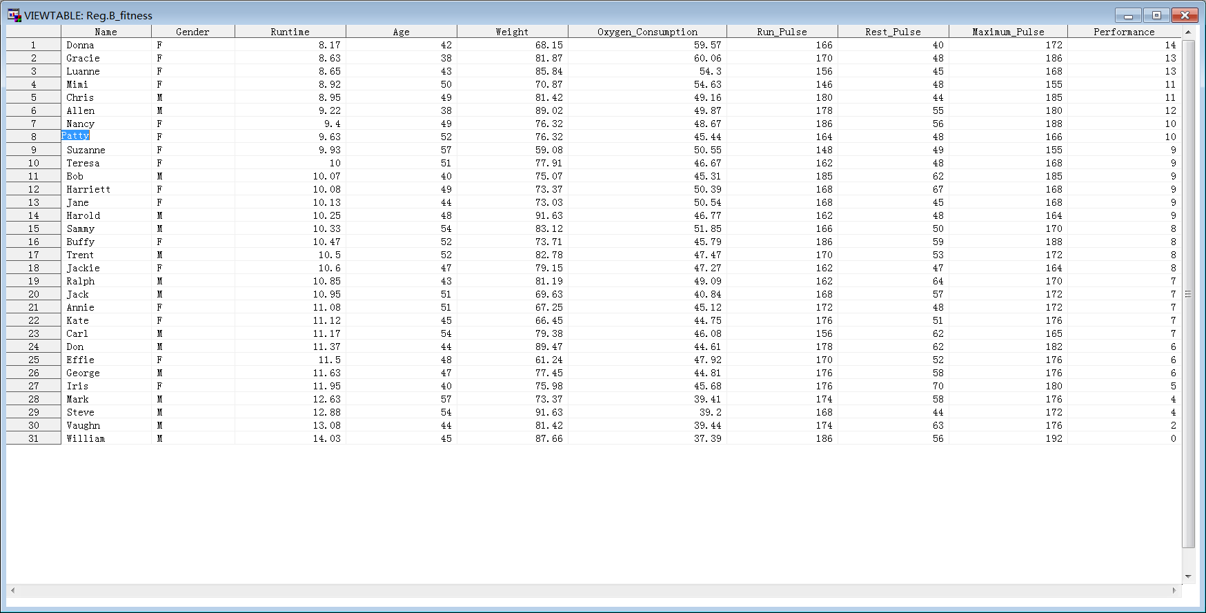
认为氧气消耗量为y变量  其余因素作为因变量

proc univariate data = reg.b_fitness;
var Runtime -- Performance;
histogram Runtime -- Performance / normal; 直方图 统计上看
probplot Runtime -- Performance / normal (mu=est sigma=est color=red w=2);  pb图  图形上看
run;

 将七个变量的直方图  pb图都画出来    如果不是正态关系 要进行正态的转换

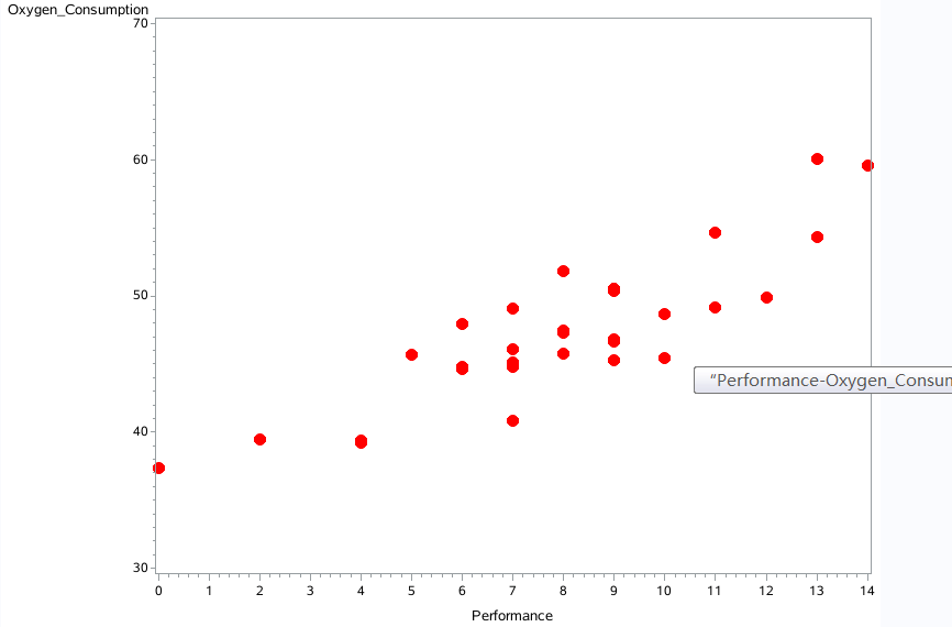
 散点图

proc gplot data = reg.b_fitness;
plot oxygen_consumption * (runtime age weight run_pulse
  rest_pulse maximum_pulse performance)
  /vaxis = axis1 haxis=axis2;
 symbol v=dot h=2 w=4 color=red;
 run;

 

相关系数

proc corr data = reg.b_fitness rank;
var runtime age weight run_pulse
  rest_pulse maximum_pulse performance;
with oxygen_consumption;  注意with with后的变量和with前变量的关系
 run;

 

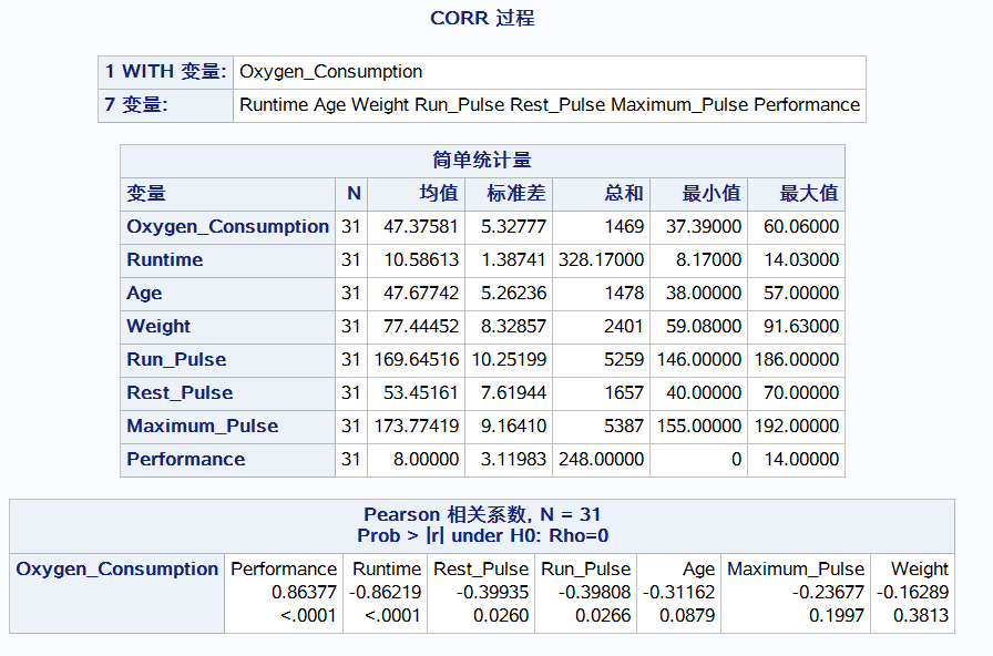
  与performance正相关相关系数0.86

 有相关关系才有必要建立回归模型

简单线性回归

 模型公式： Y = B0 + B1*X + e   其中e服从正态分布  期望值为0

零假设  B1 = 0

备选假设： B1不等于0

 

1、回归程序

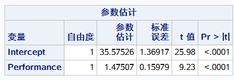
proc reg data= reg.b_fitness;
model oxygen_consumption=performance;  y变量是等号左边的 oxygen
run;

 F检验检验整个方程是否有意义

 

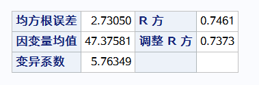
r方表示 可以解释74%的点

T检验检验系数B有没有意义    下图pvalue显示都有意义

 

2、预测值和置信区间

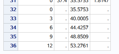
data need_predictions;
input performance @@;
datalines;
0 3 6 9 12
;
run;
第一步data步 将数据 0 3 6 9 12保存在need_predictions表中
data predoxy;
set reg.b_fitness
need_predictions;
run;
第二步data步   将原数据集和需要预测的数据集合并
proc reg data = predoxy;
model oxygen_consumption = performance / p;  p表示预测的意思
id performance;
run;

 

点估计的置信区间

proc reg data = predoxy;   
model oxygen_consumption = performance / clm cli alpha=.05;
id name performance;
plot oxygen_consumption*performance / conf pred;
symbol1 c =red v=dot;
symbol2 c =red;
symbol3 c =blue;
symbol4 c =blue;
symbol5 c =green;
symbol6 c =green;
run;

clm总体均值的置信区间

cli 观测值的置信区间   alpha 置信度水平

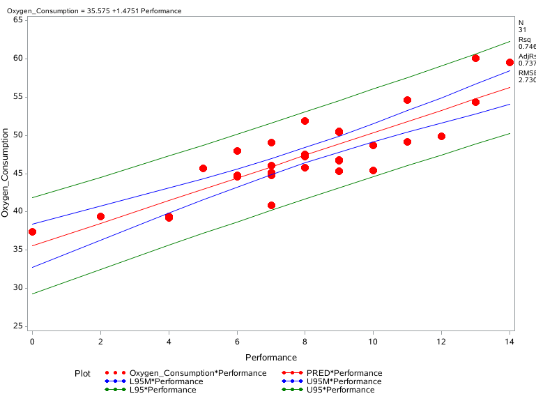
红线 线性方程 蓝线 均值置信区间   绿线 预测值 置信区间