以一元及二元函数为例，通过多项式的函数图像观察其拟合性能；以及对用多项式作目标函数进行机器学习时的一些理解。

先给出代码：

import numpy as np
from mpl_toolkits.mplot3d import Axes3D
from matplotlib import pyplot as plt
from datetime import datetime

t0 = datetime.now()
# 实数范围内非负数有偶次方根，任何实数有奇次方根；但python中负数没有奇次方根和偶次方根。
x = np.arange(-10, 10.1, 1)  

y1 = x ** 1; y2 = x ** 3; y3 = x ** 5
y4 = x ** 2; y5 = x ** 4; y6 = x ** (-1)
y7 = x ** (-3); y8 = x ** (-2); y9 = x ** (-4)

plt.subplot(331)
plt.title('y = x')
plt.plot(x, y1)
plt.subplot(332)
plt.title('y = x^3')
plt.plot(x, y2)
plt.subplot(333)
plt.title('y = x^5')
plt.plot(x, y3)
plt.subplot(334)
plt.title('y = x^2')
plt.plot(x, y4)
plt.subplot(335)
plt.title('y = x^4')
plt.plot(x, y5)
plt.subplot(336)
plt.title('y = x^(-1)')
plt.plot(x, y6)
plt.subplot(337)
plt.title('y = x^(-3)')
plt.plot(x, y7)
plt.subplot(338)
plt.title('y = x^(-2)')
plt.plot(x, y8)
plt.subplot(339)
plt.title('y = x^(-4)')
plt.plot(x, y9)
plt.show()

y10 = x ** (3/2); y11 = x ** (5/2); y12 = x ** (2/5)
y13 = x ** (4/5); y14 = x ** (-3/2); y15 = x ** (-5/2)
y16 = x ** (-2/5); y17 = (-x) ** (3/2); y18 = -(x ** (3/2))

plt.subplot(331)
plt.title('y = x^(3/2)')
plt.plot(x, y10)
plt.subplot(332)
plt.title('y = x^(5/2)')
plt.plot(x, y11)
plt.subplot(333)
plt.title('y = x^(2/5)')
plt.plot(x, y12)
plt.subplot(334)
plt.title('y = x^(4/5)')
plt.plot(x, y13)
plt.subplot(335)
plt.title('y = x^(-3/2)')
plt.plot(x, y14)
plt.subplot(336)
plt.title('y = x^(-5/2)')
plt.plot(x, y15)
plt.subplot(337)
plt.title('y = x^(-2/5)')
plt.plot(x, y16)
plt.subplot(338)
plt.title('y = (-x)^(3/2)')
plt.plot(x, y17)
plt.subplot(339)
plt.title('y = -(x^(3/2))')
plt.plot(x, y18)
plt.show()

y19 = x**2 + x; y20 = x**2 + 100*x; y21 = x**3 + x**2 + x
y22 = x**3 + 100*x**2 + x; y23 = x**4 + x**3 + x**2 + x; y24 = x**4 + 100*x**3 + x**2 + x

plt.subplot(231)
plt.title('y = x^(3/2)')
plt.plot(x, y19)
plt.subplot(232)
plt.title('y = x^(5/2)')
plt.plot(x, y20)
plt.subplot(233)
plt.title('y = x^(2/5)')
plt.plot(x, y21)
plt.subplot(234)
plt.title('y = x^(4/5)')
plt.plot(x, y22)
plt.subplot(235)
plt.title('y = x^(-3/2)')
plt.plot(x, y23)
plt.subplot(236)
plt.title('y = x^(-5/2)')
plt.plot(x, y24)
plt.show()

W = np.arange(-100, 100+0.1, 10)
B = np.arange(-100, 100+0.1, 10)
W, B = np.meshgrid(W, B)  
n = 11
for a in range(1, n, 3):
    for b in range(1, n, 3):
        for c in range(1, n, 3):
            fig = plt.figure()
            ax = Axes3D(fig)
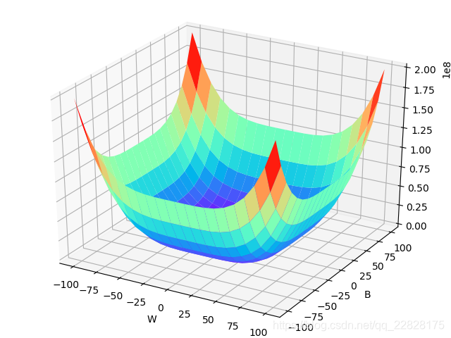
            Z = W ** a + B ** b - W * B * c
            plt.xlabel('W')
            plt.ylabel('B')
            ax.plot_surface(W, B, Z, rstride=1, cstride=1, cmap='rainbow')
            plt.show()

t1 = datetime.now()
print('总耗时：', t1-t0)

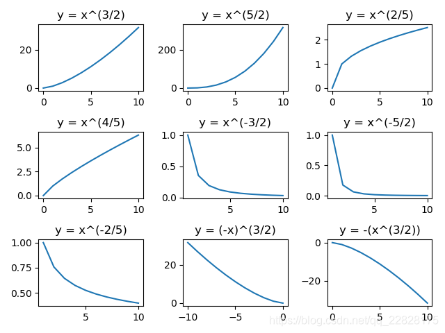
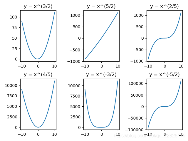
从前两张图可以看到当多项式为一元函数且没有常数项时，其自变量的幂指数依次为正奇数、正偶数、负奇数、负偶数、正假分数、正真分数、负假分数、负真分数时的函数图像。其中当幂指数为正负奇数时，函数图像关于原点对称，为奇函数；当幂指数为正负偶数时，函数图像关于纵坐标对称，为偶函数；当幂指数为正假分数时，函数单调递增且二阶导数大于0；当幂指数为正真分数时，函数单调递增且二阶导数小于0；当幂指数为负假分数、负真分数时，函数单调递减且二阶导数小于0。

从第三张图并结合其代码可以知道，多项式中哪一项分配的权重越大，函数就越会表现出那一项的性质；一般地，如果每一项权重相等，则会表现出最高次项的特征，因为高次项天然具有更大的影响力。就像在梯度下降类的算法中，高次项天然具有更高的权重。所以应当慎用高次项，避免模型过拟合。

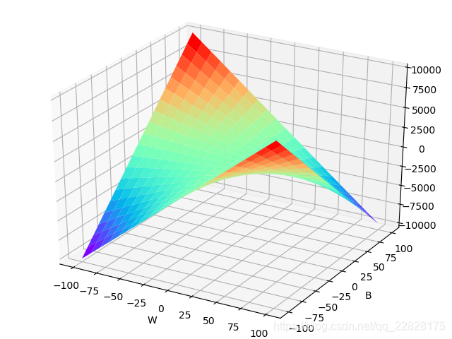
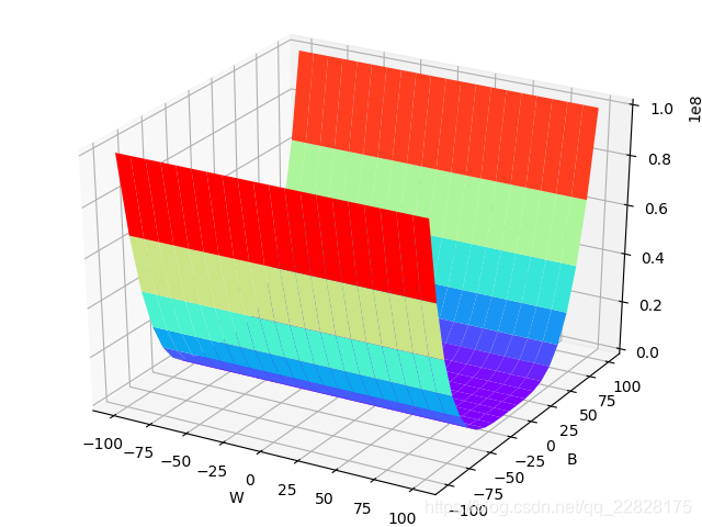
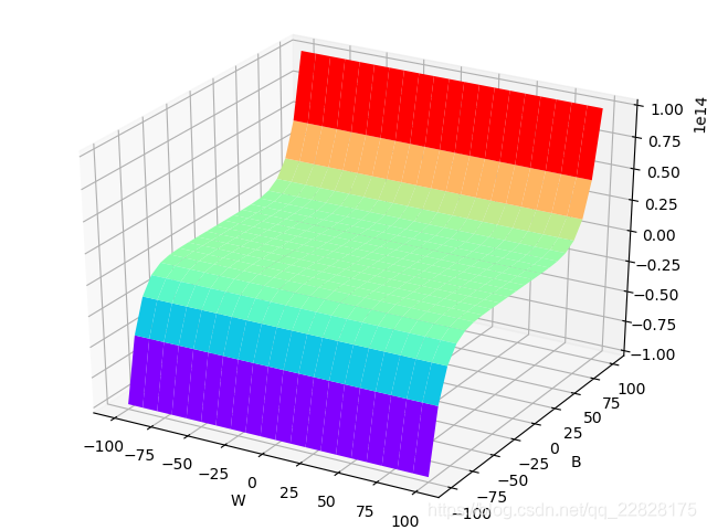
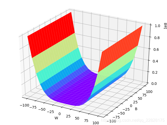
从二元函数的以上图像可以知道，如果再进行叠加，例如第一种类型的函数和第五种类型的函数叠加，或者第二种类型的函数和第四种类型的函数叠加，则函数可以拟合的数据类型会大大增加，可以分类的数据类型也会大大增加。

通过以上分析观察可以推知，如果多项式中自变量的次数没有限制，则其可以拟合及分类的数据类型非常多。但因为高次项天然具有更高的权重，在使用梯度下降类算法迭代自变量的系数时会产生巨大的跳跃，容易导致算法不收敛；就算收敛了，最终得到的多项式也容易过拟合。所以多项式最好不用高次项，如果要用，则自变量最值的绝对值不能过大；然后对自变量的系数进行迭代的时候最好加上一些降低过拟合的方法如权重衰减等。

以一元及二元函数为例，通过多项式的函数图像观察其拟合性能；以及对用多项式作目标函数进行机器学习时的一些理解。

猜你喜欢