稀疏编码中的正交匹配追踪（OMP）与代码

分享一下我老师大神的人工智能教程！零基础，通俗易懂！http://blog.csdn.net/jiangjunshow

也欢迎大家转载本篇文章。分享知识，造福人民，实现我们中华民族伟大复兴！

               

分类： AI and Computer Vision 2013-04-19 19:42 908人阅读 评论(11) 收藏 举报

OpenCV 压缩感知 稀疏编码 匹配追踪 算法

最近在看有关匹配追踪与相关优化的文章，发现了这篇http://blog.csdn.net/scucj/article/details/7467955，感觉作者写得很不错，这里也再写写自己的理解。文中有Matlab的代码，为了方便以后的使用，我顺便写了一个C++版本的，方便与OpenCV配合。

为了方便理解，我将所有向量都表示为平面二维向量，待用原子表征的目标向量y，用红色表示，原子向量用蓝色表示，残差向量用绿色表示。于是匹配追踪算法（MP）实际上可以用下图表示。

注意原子向量和目标向量都已归一化到单位长度，MP算法首先在所有原子向量中找到向OA投影最大的向量，即OB，然后计算OA - <OA, OB>OB，其中的<OA, OB>OB也就是图中的OD了，被OA减掉后，剩下的就是残差DA，根据初中几何知识就可以知道，DA是一定垂直于OB的，也就是说MP的残差始终与最近选出来的那个原子向量正交。

而OMP要做的，就是让残差与已经选出来的所有原子向量都正交，这一点在图上不好画出来，但上面的那篇博文写的已经很详尽了，这里不再敖述。

下面是用C++实现的OMP算法，具体流程参考上面博文中的一张图：

其中的最小二乘可以直接通过矩阵运算得到，也可以使用OpenCV的solve方法，该方法专门用于求解线性方程组或最小二乘问题。代码如下：

void OrthMatchPursuit( vector<Mat>& dic,//字典 Mat& target,  float min_residual,  int sparsity,  Mat& x,  //返回每个原子对应的系数; vector<int>& patch_indices  //返回选出的原子序号 ){ Mat residual = target.clone();  Mat phi; //保存已选出的原子向量 x.create(0, 1, CV_32FC1);  float max_coefficient; unsigned int patch_index; for(;;) {  max_coefficient = 0;  for (int i = 0; i < dic.size(); i++)  {   float coefficient = (float)dic[i].dot(residual);    if (abs(coefficient) > abs(max_coefficient))   {   max_coefficient = coefficient;   patch_index = i;   }  }  patch_indices.push_back(patch_index); //添加选出的原子序号    Mat& matched_patch = dic[patch_index];  if (phi.cols == 0)   phi = matched_patch;  else   hconcat(phi,matched_patch,phi); //将新原子合并到原子集合中（都是列向量）    x.push_back(0.0f); //对系数矩阵新加一项  solve(phi, target, x, DECOMP_SVD); //求解最小二乘问题  residual = target - phi*x;  //更新残差  float res_norm = (float)norm(residual);  if (x.rows >= sparsity || res_norm <= min_residual) //如果残差小于阈值或达到要求的稀疏度，就返回   return; }}

代码写得有点乱，基本上完全按照算法步骤来的，应该还有很大的性能提升空间。

===================================无耻的分割线========================================

之前说上面的代码还有很大的优化空间，这几天捣鼓了一下，发现优化还是很有成效的，下面是具体方法。

为方便起见，这里用A代表从字典当中选出的原子的集合，对于上面求解最小二乘的一步，可以表示为下式：

其中的是一个对称正定矩阵，现在假如经过一次搜索后，又找到了一个原子向量v，那么新的原子集合可以表示为：

那么用这个新的原子集合计算x时，可以得到：

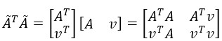
可以看到，新的集合乘积，有一部分是上次的结果（上式最右边矩阵的第一个元素），因此没有必要每次都从新计算，而只需对原来的矩阵更新一列和一行就行了。同时，上式的第二和第三个元素互为转置，也只需要计算其中一个，第四个元素是v的二范数的平方，直接调用norm()函数求得。

在对矩阵进行行和列的添加时，我放弃了使用vconcat和hconcat方法，这两个方法效率较低，每次添加都会把原来的部分复制一遍。我现在一次分配好需要的大小，然后通过Mat的括号操作符取需要的子矩阵进行更新和计算。

求解x时，还有一步是求的逆，既然是对称正定的，可以进行Cholesky分解，那么它的逆也可以很快求出。刚好OpenCV中有这样的方法，即调用inv()方法时，用DECOMP_CHOLESKY作为参数，根据官方文档，这样的速度是普通矩阵求逆的两倍！

我做了一个测试，使用一个有600多个原子的字典，每个原子的维度为200，稀疏度设定为10，匹配一个信号，原来的方法需要200ms左右，而用上面的方法优化后，只需10ms！！快了一个数量级！！

下面是优化后的代码：

void DictionaryLearning::OrthMatchPursuit( Mat& target,  float min_residual,  int sparsity, //Store matched patches' coefficient vector<float>& coefficients,  //Store matched patches vector<DicPatch>& matched_patches, //Store indices of matched patches vector<int>& matched_indices ){ Mat residual = target.clone();  //the atoms' set; Mat ori_phi = Mat::zeros(m_vec_dims,sparsity,CV_32FC1); Mat phi; //phi.t()*phi which is a SPD matrix Mat ori_spd = Mat::ones(sparsity,sparsity,CV_32FC1); Mat spd = ori_spd(Rect(0,0,1,1));  //reserve enough memory. matched_patches.reserve(sparsity); matched_indices.reserve(sparsity); float max_coefficient; int matched_index; deque<DicPatch>::iterator matched_patch_it;  for(int spars = 1;;spars++) {  max_coefficient = 0;  matched_index = 0;  int current_index = 0;  for (deque<DicPatch>::iterator patch_it = m_patches.begin();    patch_it != m_patches.end();    ++patch_it   )  {   Mat& cur_vec = (*patch_it).vector;   float coefficient = (float)cur_vec.dot(residual);    //Find the maxmum coefficient   if (abs(coefficient) > abs(max_coefficient))   {    max_coefficient = coefficient;    matched_patch_it = patch_it;    matched_index = current_index;   }   current_index++;  }  matched_patches.push_back((*matched_patch_it));  matched_indices.push_back(matched_index);    Mat& matched_vec = (*matched_patch_it).vector;    //update the spd matrix via symply appending a single row and column to it.  if (spars > 1)  {   Mat v = matched_vec.t()*phi;   float c = (float)norm(matched_vec);   Mat new_row = ori_spd(Rect(0, spars - 1, spars - 1, 1));   Mat new_col = ori_spd(Rect(spars - 1, 0, 1, spars - 1));   v.copyTo(new_row);   ((Mat)v.t()).copyTo(new_col);   *ori_spd.ptr<float>(spars - 1, spars - 1) = c*c;   spd = ori_spd(Rect(0, 0, spars, spars));  }  //Add the new matched patch to the vectors' set.  phi = ori_phi(Rect(0, 0, spars, m_vec_dims));  matched_vec.copyTo(phi.col(spars - 1));     //A SPD matrix! Use Cholesky process to speed up.  Mat x = spd.inv(DECOMP_CHOLESKY)*phi.t()*target;  residual = target - phi*x;    float res_norm = (float)norm(residual);  if (spars >= sparsity || res_norm <= min_residual)  {   coefficients.clear();   coefficients.reserve(x.cols);   x.copyTo(coefficients);   return;  } }}

           

给我老师的人工智能教程打call！http://blog.csdn.net/jiangjunshow

最近在看有关匹配追踪与相关优化的文章，发现了这篇http://blog.csdn.net/scucj/article/details/7467955，感觉作者写得很不错，这里也再写写自己的理解。文中有Matlab的代码，为了方便以后的使用，我顺便写了一个C++版本的，方便与OpenCV配合。

为了方便理解，我将所有向量都表示为平面二维向量，待用原子表征的目标向量y，用红色表示，原子向量用蓝色表示，残差向量用绿色表示。于是匹配追踪算法（MP）实际上可以用下图表示。

注意原子向量和目标向量都已归一化到单位长度，MP算法首先在所有原子向量中找到向OA投影最大的向量，即OB，然后计算OA - <OA, OB>OB，其中的<OA, OB>OB也就是图中的OD了，被OA减掉后，剩下的就是残差DA，根据初中几何知识就可以知道，DA是一定垂直于OB的，也就是说MP的残差始终与最近选出来的那个原子向量正交。

而OMP要做的，就是让残差与已经选出来的所有原子向量都正交，这一点在图上不好画出来，但上面的那篇博文写的已经很详尽了，这里不再敖述。

下面是用C++实现的OMP算法，具体流程参考上面博文中的一张图：

其中的最小二乘可以直接通过矩阵运算得到，也可以使用OpenCV的solve方法，该方法专门用于求解线性方程组或最小二乘问题。代码如下：

void OrthMatchPursuit( vector<Mat>& dic,//字典 Mat& target,  float min_residual,  int sparsity,  Mat& x,  //返回每个原子对应的系数; vector<int>& patch_indices  //返回选出的原子序号 ){ Mat residual = target.clone();  Mat phi; //保存已选出的原子向量 x.create(0, 1, CV_32FC1);  float max_coefficient; unsigned int patch_index; for(;;) {  max_coefficient = 0;  for (int i = 0; i < dic.size(); i++)  {   float coefficient = (float)dic[i].dot(residual);    if (abs(coefficient) > abs(max_coefficient))   {   max_coefficient = coefficient;   patch_index = i;   }  }  patch_indices.push_back(patch_index); //添加选出的原子序号    Mat& matched_patch = dic[patch_index];  if (phi.cols == 0)   phi = matched_patch;  else   hconcat(phi,matched_patch,phi); //将新原子合并到原子集合中（都是列向量）    x.push_back(0.0f); //对系数矩阵新加一项  solve(phi, target, x, DECOMP_SVD); //求解最小二乘问题  residual = target - phi*x;  //更新残差  float res_norm = (float)norm(residual);  if (x.rows >= sparsity || res_norm <= min_residual) //如果残差小于阈值或达到要求的稀疏度，就返回   return; }}

代码写得有点乱，基本上完全按照算法步骤来的，应该还有很大的性能提升空间。

===================================无耻的分割线========================================

之前说上面的代码还有很大的优化空间，这几天捣鼓了一下，发现优化还是很有成效的，下面是具体方法。

为方便起见，这里用A代表从字典当中选出的原子的集合，对于上面求解最小二乘的一步，可以表示为下式：

其中的是一个对称正定矩阵，现在假如经过一次搜索后，又找到了一个原子向量v，那么新的原子集合可以表示为：

那么用这个新的原子集合计算x时，可以得到：

可以看到，新的集合乘积，有一部分是上次的结果（上式最右边矩阵的第一个元素），因此没有必要每次都从新计算，而只需对原来的矩阵更新一列和一行就行了。同时，上式的第二和第三个元素互为转置，也只需要计算其中一个，第四个元素是v的二范数的平方，直接调用norm()函数求得。

在对矩阵进行行和列的添加时，我放弃了使用vconcat和hconcat方法，这两个方法效率较低，每次添加都会把原来的部分复制一遍。我现在一次分配好需要的大小，然后通过Mat的括号操作符取需要的子矩阵进行更新和计算。

求解x时，还有一步是求的逆，既然是对称正定的，可以进行Cholesky分解，那么它的逆也可以很快求出。刚好OpenCV中有这样的方法，即调用inv()方法时，用DECOMP_CHOLESKY作为参数，根据官方文档，这样的速度是普通矩阵求逆的两倍！

我做了一个测试，使用一个有600多个原子的字典，每个原子的维度为200，稀疏度设定为10，匹配一个信号，原来的方法需要200ms左右，而用上面的方法优化后，只需10ms！！快了一个数量级！！

下面是优化后的代码：

void DictionaryLearning::OrthMatchPursuit( Mat& target,  float min_residual,  int sparsity, //Store matched patches' coefficient vector<float>& coefficients,  //Store matched patches vector<DicPatch>& matched_patches, //Store indices of matched patches vector<int>& matched_indices ){ Mat residual = target.clone();  //the atoms' set; Mat ori_phi = Mat::zeros(m_vec_dims,sparsity,CV_32FC1); Mat phi; //phi.t()*phi which is a SPD matrix Mat ori_spd = Mat::ones(sparsity,sparsity,CV_32FC1); Mat spd = ori_spd(Rect(0,0,1,1));  //reserve enough memory. matched_patches.reserve(sparsity); matched_indices.reserve(sparsity); float max_coefficient; int matched_index; deque<DicPatch>::iterator matched_patch_it;  for(int spars = 1;;spars++) {  max_coefficient = 0;  matched_index = 0;  int current_index = 0;  for (deque<DicPatch>::iterator patch_it = m_patches.begin();    patch_it != m_patches.end();    ++patch_it   )  {   Mat& cur_vec = (*patch_it).vector;   float coefficient = (float)cur_vec.dot(residual);    //Find the maxmum coefficient   if (abs(coefficient) > abs(max_coefficient))   {    max_coefficient = coefficient;    matched_patch_it = patch_it;    matched_index = current_index;   }   current_index++;  }  matched_patches.push_back((*matched_patch_it));  matched_indices.push_back(matched_index);    Mat& matched_vec = (*matched_patch_it).vector;    //update the spd matrix via symply appending a single row and column to it.  if (spars > 1)  {   Mat v = matched_vec.t()*phi;   float c = (float)norm(matched_vec);   Mat new_row = ori_spd(Rect(0, spars - 1, spars - 1, 1));   Mat new_col = ori_spd(Rect(spars - 1, 0, 1, spars - 1));   v.copyTo(new_row);   ((Mat)v.t()).copyTo(new_col);   *ori_spd.ptr<float>(spars - 1, spars - 1) = c*c;   spd = ori_spd(Rect(0, 0, spars, spars));  }  //Add the new matched patch to the vectors' set.  phi = ori_phi(Rect(0, 0, spars, m_vec_dims));  matched_vec.copyTo(phi.col(spars - 1));     //A SPD matrix! Use Cholesky process to speed up.  Mat x = spd.inv(DECOMP_CHOLESKY)*phi.t()*target;  residual = target - phi*x;    float res_norm = (float)norm(residual);  if (spars >= sparsity || res_norm <= min_residual)  {   coefficients.clear();   coefficients.reserve(x.cols);   x.copyTo(coefficients);   return;  } }}