%% logspace
A=linspace(1,6)%从1到6一共100个数
A1=logspace(1,6)%从10^1到10^6一共50个数,默认生成100个数
A2=logspace(1,6,100)%从10^1到10^6一共100个数
A3=logspace(1,pi)%生成的是10到pi的一共50个数,若写成3.1415926535……生成的不是pi
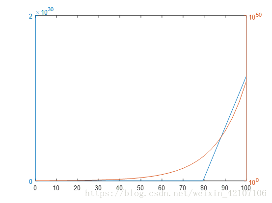
%% loglog
Y=[1 5 10 25 40 60 80 100];
% loglog(Y);
x=10.^(-1:0.1:2)
y=2.^x;
% subplot(1,2,1)
% h=loglog(x,y,'--dr','Markersize',2)
% subplot(1,2,2)
% plot(x,y)
plotyy(x,y,x,y,'plot','loglog') %图二显示

%% semilogx
%X轴是对数,Y轴是线性
x=10.^(-1:0.5:2)
y=x+1./x;
semilogx(x,y)
%% semilogy
%X轴是线性,Y轴是对数
%% 匿名函数
% f=@(x) sin(x)+cos(x);
% f(pi/2)
% f1=@(x,y) sin(x)+cos(y)
% f1(pi/2,pi/3)
% f2=@(x,y) @(a) sin(x)+cos(y)+a;
% % f2(pi/2,pi/3,1)%出错
% f3=f2(pi/2,pi/3);
% f3(1)
% f=@(x) x.^2+2
% fplot(f)%默认的x轴坐标范围为-5到5
% fplot(f,[-2,2])
%fplot('sin(x)',[-2*pi,2*pi])%在以后的版本中会删除
% fplot(@(x)sin(x),[-pi,pi])
%% 参数方程
% x=@(t) cos(3*t);
% y=@(t) sin(5*t);
% fplot(x,y)
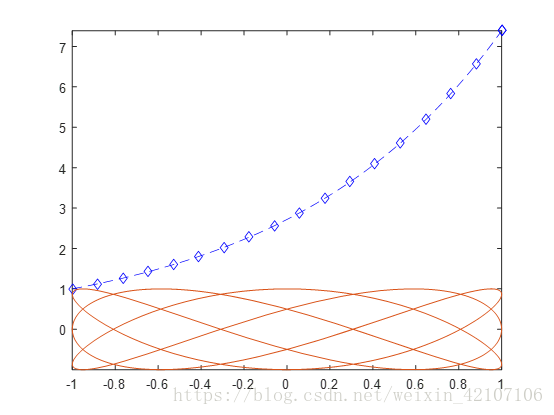
%% e怎么输入exp()
fplot(@(x)exp(x+1),[-1,1],'--bd')
hold on
%% 句柄
x=@(t) cos(3*t);
y=@(t) sin(5*t);
fp=fplot(x,y);
fp.MarkerSize=3;
%% ezplot easyplot
% ezplot('x^3+x^2+2') %默认范围是【-2*pi 2*pi】
% ezplot('x^3+x^2+2',[-5,5])
%匿名函数句柄
% f=@(x) x.^2
% ezplot(f)
%隐函数 e^x+y^2-2=0
% ezplot('exp(x)+y^2-2=0',[-5 5 -5 4])
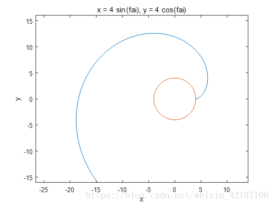
%参数方程绘图
syms fai %定义符号变量fai
r=input('请输入半径: ')
x=r*(cos(fai)+fai*sin(fai));
y=r*(sin(fai)-fai*cos(fai));
ezplot(x,y)%这里不能使用ezplot(x,y,x1,y1)
axis([-4*r 4*r -4*r 4*r])
hold on
x1=r*sin(fai)
y1=r*cos(fai)
ezplot(x1,y1)
%% quiver(u,v)
% u=[0.1 0.3 0.5 0.6]
% v=[0.6 0.1 0.5 0.6]
% quiver(u,v)%根据u,v做出某种图线,下图一
%% quiver(x,y,u,v)
syms x y y1
y=x^3+2*x
y1=diff(y,x)%y方程中对x求导,diff()求导函数
x1=-5:0.5:5
y=double(subs(y,x,x1));%y,y1,x均为参数需转换
y1=double(subs(y1,x,x1));
sita=atan(y1)%求斜率的角度,atan相当于数学里的arctan
tx=y1.*cos(sita)
ty=y1.*sin(sita)
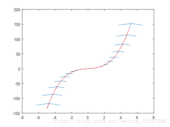
q=quiver(x1,y,tx,ty,0.3)%这里0.3是将箭头调小一点,这里箭头表示某点的斜率
hold on
plot(x1,y,'r') 下图二

%% x,y是矩阵
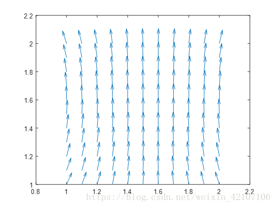
x=1:0.1:2;
y=x;
[X,Y]=meshgrid(x,y)%生成网格数据
u=cos(X).*cos(Y)
v=sin(X).*sin(Y)
quiver(X,Y,u,v)
syms x y y1
y=x^3+2*x
y1=diff(y,x)%y方程中对x求导,diff()求导函数
x1=-5:0.5:5
y=double(subs(y,x,x1));%y,y1,x均为参数需转换
y1=double(subs(y1,x,x1));
sita=atan(y1)%求斜率的角度,atan相当于数学里的arctan
tx=y1.*cos(sita)
ty=y1.*sin(sita)
p=plot(x1,y)
axis([-5 10 -150 200])%防止最后的箭头没有
hold on
xlim=get(p.Parent,'XLim')%;p.parent即是坐标轴,XLim是x轴的坐标范围,结果显示的是我们设定的【-5 5】
ylim=get(p.Parent,'YLim')
po=get(p.Parent,'position')%po = 0.1300 0.1100 0.7750 0.8150
[~,px]=mapminmax(xlim,po(1),po(1)+po(3))%将x归一化
[~,py]=mapminmax(ylim,po(2),po(2)+po(4))
xx1=mapminmax('apply',x1,px)%以px结构归一化处理x1赋值给xx1
y1=mapminmax('apply',y,py)
txx=mapminmax('apply',x1+tx,px)
tyy=mapminmax('apply',y+ty,py)
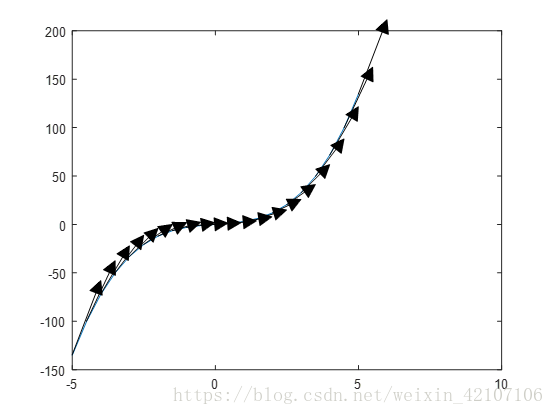
for i=1:length(x1)
p1=annotation('arrow',[xx1(i),txx(i)],[y1(i),tyy(i)],'HeadStyle','plain')%设p1看有什么属性可设置
end
%% annotation
%annotation('arrow',[0 1],[0 1])%x的起点是0,终点是1,即第一个【0 1】,同理y
% q=quiver(x1,y,tx,ty,0.3)%这里0.3是将箭头调小一点,这里箭头表示某点的斜率
%% bar
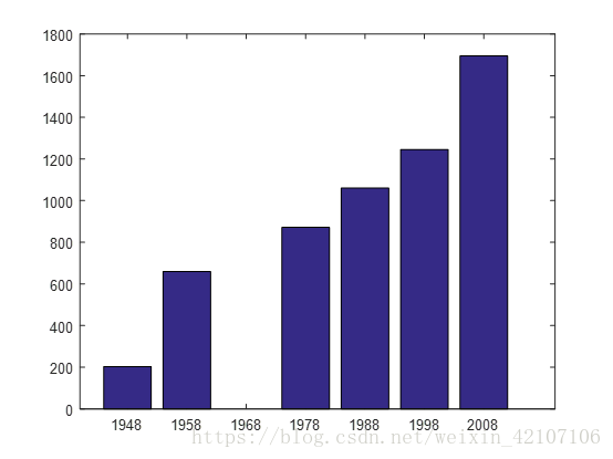
%北京1948年到2008的人口直方图bar 这里1968年无数据,用NaN表示
year=1948:10:2008;
num=[203 660 NaN 871.5 1061 1245.6 1695];
bar(year,num) 下图一
%第一种重叠绘图
% h1=gca;
% h1.Box='off';
% h2=axes('Position',get(h1,'Position'))
% plot(h2,year,num)
% h2.YAxisLocation='right';
% h2.XLim=h1.XLim;
% h2.YLim=h1.YLim;
% h2.XTick=[];%防止两者的刻度重叠混乱
% h2.XTickLabel=[];
% h2.Color='none';%不让h2的颜色遮盖掉h1的颜色 下图一
%% 第二种重叠绘图
% plotyy(year,num,year,num,'bar','plot') 下图一
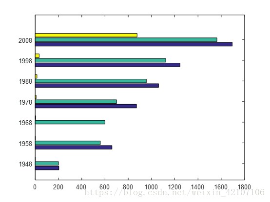
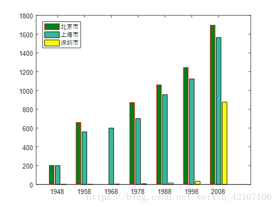
%% 北京 上海 深圳人口变换
year=1948:10:2008
num=[203 200 1.5;660 560 2;NaN 600 4;871.5 700 7.65;1061 956 15.3;1245.6 1123 34.07;1695 1563 876;];
b=bar(year,num)
hh=legend('北京市','上海市','深圳市')
hh.Location='Northwest';
b(1).EdgeColor='red';
b(1).FaceColor=[0.01 0.5 0.1] 下图二
%% barh
% close
% barh(year,num) 下图一
%% bar3
close
bar3(year,num) 下图二
xlabel('x轴')
ylabel('y轴')
zlabel('z轴')