if __name__ == "__main__":
    # # 开场白:
    # numpy是非常好用的数据包,如:可以这样得到这个二维数组
    # [[ 0  1  2  3  4  5]
    #  [10 11 12 13 14 15]
    #  [20 21 22 23 24 25]
    #  [30 31 32 33 34 35]
    #  [40 41 42 43 44 45]
    #  [50 51 52 53 54 55]]
    a = np.arange(0, 60, 10).reshape((-1, 1)) + np.arange(6)
    print(a)

    # 正式开始  -:)
    # 标准Python的列表(list)中,元素本质是对象。
    # 如:L = [1, 2, 3],需要3个指针和三个整数对象,对于数值运算比较浪费内存和CPU。
    # 因此,Numpy提供了ndarray(N-dimensional array object)对象:存储单一数据类型的多维数组。

    # # 1.使用array创建
    # 通过array函数传递list对象
    L = [1, 2, 3, 4, 5, 6]
    print("L = ", L)
    a = np.array(L)
    print("a = ", a)
    print(type(a), type(L))
    # 若传递的是多层嵌套的list,将创建多维数组
    b = np.array([[1, 2, 3, 4], [5, 6, 7, 8], [9, 10, 11, 12]])
    print(b)

    # # # # # 数组大小可以通过其shape属性获得
    print(a.shape)
    print(b.shape)

    # # 也可以强制修改shape
    b.shape = 4, 3
    print(b)
    # # 注:从(3,4)改为(4,3)并不是对数组进行转置,而只是改变每个轴的大小,数组元素在内存中的位置并没有改变
    #
    # # # 当某个轴为-1时,将根据数组元素的个数自动计算此轴的长度

    # # 数组的元素类型可以通过dtype属性获得
    print(a.dtype)
    print(b.dtype)
    # # # # #
    # # # # # 可以通过dtype参数在创建时指定元素类型
    d = np.array([[1, 2, 3, 4], [5, 6, 7, 8], [9, 10, 11, 12]], dtype=np.float)
    f = np.array([[1, 2, 3, 4], [5, 6, 7, 8], [9, 10, 11, 12]], dtype=np.complex)
    print(d.dtype)
    print(f)
    print(f.dtype)

    # # # 如果更改元素类型,可以使用astype安全的转换
    f = d.astype(np.int)
    print(f)
    # #
    # # # 但不要强制仅修改元素类型,如下面这句,将会以int来解释单精度float类型
    d.dtype = np.int
    print(d)

    # 2.使用函数创建
    # 如果生成一定规则的数据,可以使用NumPy提供的专门函数
    # arange函数类似于python的range函数:指定起始值、终止值和步长来创建数组
    # 和Python的range类似,arange同样不包括终值;但arange可以生成浮点类型,而range只能是整数类型
    np.set_printoptions(linewidth=100, suppress=True)
    a = np.arange(1, 10, 1)
    print('a = ', a)

    # # # # linspace函数通过指定起始值、终止值和元素个数来创建数组,缺省包括终止值 默认包含endpoint =true 包含。
    b = np.linspace(1, 10, 10)
    print('b = ', b)
    print(b.dtype)

    # # 可以通过endpoint关键字指定是否包括终值
    c = np.linspace(1, 10, 10, endpoint=False, dtype=np.int32)
    print('c = ', c)
    print(c.dtype)

    # # # 和linspace类似,logspace可以创建等比数列
    # # 下面函数创建起始值为10^1,终止值为10^2,有10个数的等比数列
    d = np.logspace(1, 4, 4, endpoint=True, base=2)
    print(d)

    # # # # # 下面创建起始值为2^0,终止值为2^10(包括),有10个数的等比数列
    np.set_printoptions(linewidth=100, suppress=True)
    f = np.logspace(0, 10, 11, endpoint=True, base=2)
    print(f)

    # # # # 使用 frombuffer, fromstring, fromfile等函数可以从字节序列创建数组
    s = 'abcdzzzz'
    g = np.fromstring(s, dtype=np.int8)
    print(g)
    # [ 97  98  99 100 122 122 122 122]

    # # 3.存取
    # 3.1常规办法:数组元素的存取方法和Python的标准方法相同
    a = np.arange(10)
    print(a)
    # # # 获取某个元素
    print(a[3])
    # # # # # 切片[3,6),左闭右开
    print(a[3:6])
    # # # 省略开始下标,表示从0开始
    print(a[:5])
    # # # 下标为负表示从后向前数
    print(a[3:])
    # # 步长为2
    print(a[1:9:2])
    # # # # # # 步长为-1,即翻转
    print(a[::-1])
    # # 切片数据是原数组的一个视图,与原数组共享内容空间,可以直接修改元素值
    a[1:4] = 10, 20, 30
    print(a)
    # # 因此,在实践中,切实注意原始数据是否被破坏,如:
    b = a[2:5]
    b[0] = 200
    print(b)
    print(a)

    # 3.2 整数/布尔数组存取
    # 3.2.1
    # 根据整数数组存取:当使用整数序列对数组元素进行存取时,
    # 将使用整数序列中的每个元素作为下标,整数序列可以是列表(list)或者数组(ndarray)。
    # 使用整数序列作为下标获得的数组不和原始数组共享数据空间。
    a = np.logspace(0, 9, 10, base=2)
    print(a)
    i = np.arange(0, 10, 2)
    print(i)
    # # 利用i取a中的元素
    b = a[i]
    print(b)
    # # b的元素更改,a中元素不受影响
    b[2] = 1.6
    print(b)
    print(a)

    # # 3.2.2
    # 使用布尔数组i作为下标存取数组a中的元素:返回数组a中所有在数组b中对应下标为True的元素
    # 生成10个满足[0,1)中均匀分布的随机数
    np.set_printoptions(linewidth=200, suppress=True)
    a = np.random.rand(10)
    print(a)
    # # 大于0.5的元素索引
    print('a > 0.5 =', a > 0.5)
    # # # 大于0.5的元素
    b = a[a > 0.5]
    print('a[a > 0.5]=', b)
    # # # 将原数组中大于0.5的元素截取成0.5
    a[a > 0.5] = 0.5
    print('a[a > 0.5] = 0.5', a)
    # # # # # b不受影响
    print(b)

    # 3.3 二维数组的切片
    # [[ 0  1  2  3  4  5]
    #  [10 11 12 13 14 15]
    #  [20 21 22 23 24 25]
    #  [30 31 32 33 34 35]
    #  [40 41 42 43 44 45]
    #  [50 51 52 53 54 55]]
    a = np.arange(0, 60, 10)    # 行向量
    print('a = ', a)
    b = a.reshape((-1, 1))      # 转换成列向量
    print(b)
    c = np.arange(6)
    print(c)
    f = b + c   # 行 + 列
    print(f)
    # 合并上述代码:
    a = np.arange(0, 60, 10).reshape((-1, 1)) + np.arange(6)
    print(a)
    # # 二维数组的切片
    print(a[[0, 1, 2], [2, 3, 4]])
    print(a[4, [2, 3, 4]])
    print(a[4:, [2, 3, 4]])
    i = np.array([True, False, True, False, False, True])
    print(a[i])
    print(a[i, 3])

    # 4.1 numpy与Python数学库的时间比较,大概是numpy是python 20分之一
    for j in np.logspace(0, 7, 8):
        x = np.linspace(0, 10, j)
        start = time.clock()
        y = np.sin(x)
        t1 = time.clock() - start

        x = x.tolist()
        start = time.clock()
        for i, t in enumerate(x):
            x[i] = math.sin(t)
        t2 = time.clock() - start
        print(j, ": ", t1, t2, t2/t1)

    # 4.2 元素去重
    # 4.2.1直接使用库函数
    a = np.array((1, 2, 3, 4, 5, 5, 7, 3, 2, 2, 8, 8))
    # print('原始数组:', a)
    # # 使用库函数unique
    # b = np.unique(a)
    # print('去重后:', b)
    # # 4.2.2 二维数组的去重,结果会是预期的么?
    # c = np.array(((1, 2), (3, 4), (5, 6), (1, 3), (3, 4), (7, 6)))
    # print('二维数组:\n', c)
    # print('去重后:', np.unique(c))
    # # # 4.2.3 方案1:转换为虚数
    # r, i = np.split(c, (1, ), axis=1)
    # x = r + i * 1j
    # # x = c[:, 0] + c[:, 1] * 1j
    # print('转换成虚数:', x)
    # print('虚数去重后:', np.unique(x))
    # print(np.unique(x, return_index=True))   # 思考return_index的意义
    # idx = np.unique(x, return_index=True)[1]
    # print('二维数组去重:\n', c[idx])
    # 4.2.3 方案2:利用set    (最好)
    print('去重方案2:\n', np.array(list(set([tuple(t) for t in c]))))

    # 4.3 stack and axis 很重要 在图片的拼接上可以使得代码简短
    a = np.arange(1, 7).reshape((2, 3))
    b = np.arange(11, 17).reshape((2, 3))
    c = np.arange(21, 27).reshape((2, 3))
    d = np.arange(31, 37).reshape((2, 3))
    print('a = \n', a)
    print('b = \n', b)
    print('c = \n', c)
    print('d = \n', d)
    s = np.stack((a, b, c, d), axis=0)
    print('axis = 0 ', s.shape, '\n', s)
    s = np.stack((a, b, c, d), axis=1)
    print('axis = 1 ', s.shape, '\n', s)
    s = np.stack((a, b, c, d), axis=2)
    print('axis = 2 ', s.shape, '\n', s)

    a = np.arange(1, 10).reshape(3,3)
    print(a)
    b = a + 10
    print(b)
    print(np.dot(a, b))
    print(a * b)

    a = np.arange(1, 10)
    print(a)
    b = np.arange(20,25)
    print(b)
    print(np.concatenate((a, b)))


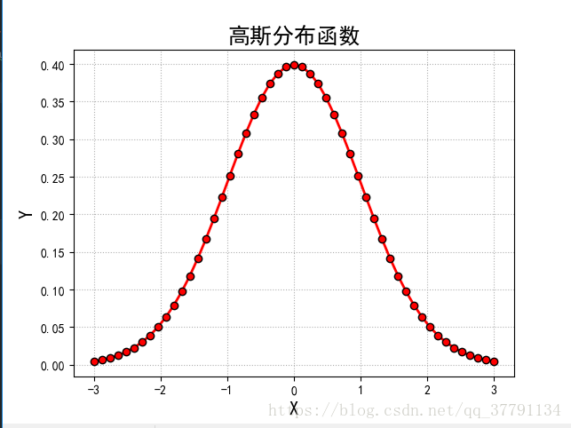
 # 5.1 绘制正态分布概率密度函数
    mpl.rcParams['font.sans-serif'] = [u'SimHei']  #FangSong/黑体 FangSong/KaiTi  没有它的话“高斯分布函数”文字出不来
    mpl.rcParams['axes.unicode_minus'] = False #不要解码英文
    mu = 0
    sigma = 1
    x = np.linspace(mu - 3 * sigma, mu + 3 * sigma, 51)
    y = np.exp(-(x - mu) ** 2 / (2 * sigma ** 2)) / (math.sqrt(2 * math.pi) * sigma)
    print(x.shape)
    print('x = \n', x)
    print(y.shape)
    print('y = \n', y)
    plt.figure(facecolor='w')
    plt.plot(x, y, 'ro-', linewidth=2, markeredgecolor='k')
    # plt.plot(x, y, 'r-', x, y, 'go', linewidth=2, markersize=8)
    plt.xlabel('X', fontsize=15)
    plt.ylabel('Y', fontsize=15)
    plt.title(u'高斯分布函数', fontsize=18)    #
    plt.grid(True, linestyle=':')
    plt.show()
  # 5.2 损失函数:Logistic损失(-1,1)/SVM Hinge损失/ 0/1损失
    plt.figure(figsize=(10, 8))
    x = np.linspace(start=-2, stop=3, num=1001, dtype=np.float)
    y_logit = np.log(1 + np.exp(-x)) / math.log(2)
    y_boost = np.exp(-x)
    y_01 = x < 0
    y_hinge = 1.0 - x
    y_hinge[y_hinge < 0] = 0
    plt.plot(x, y_logit, 'r-', label='Logistic Loss', linewidth=2)
    plt.plot(x, y_01, 'g-', label='0/1 Loss', linewidth=2)
    plt.plot(x, y_hinge, 'b-', label='Hinge Loss', linewidth=2)
    plt.plot(x, y_boost, 'm--', label='Adaboost Loss', linewidth=2)
    plt.grid()
    plt.legend(loc='upper right')
    # plt.savefig('1.png')
    plt.show()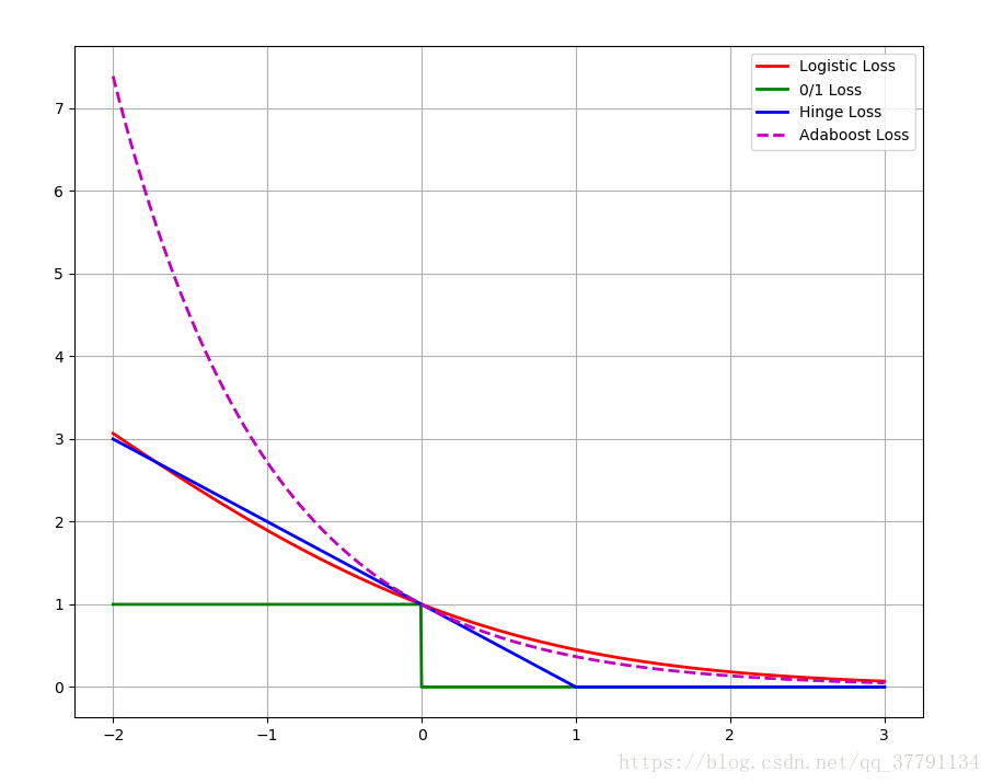
  # 5.3 x^x
    plt.figure(facecolor='w')
    x = np.linspace(-1.3, 1.3, 101)
    y = f(x)
    plt.plot(x, y, 'g-', label='x^x', linewidth=2)
    plt.grid(True, ls='--')
    plt.legend(loc='upper left')
    plt.show()

 # 5.4 胸型线
    x = np.arange(1, 0, -0.001)
    y = (-3 * x * np.log(x) + np.exp(-(40 * (x - 1 / np.e)) ** 4) / 25) / 2
    plt.figure(figsize=(5,7), facecolor='w')
    plt.plot(y, x, 'r-', linewidth=2)
    plt.grid(True)
    plt.title(u'胸型线', fontsize=20)
    # plt.savefig('breast.png')
    plt.show()
# 5.5 心形线
    t = np.linspace(0, 2*np.pi, 100)
    x = 16 * np.sin(t) ** 3
    y = 13 * np.cos(t) - 5 * np.cos(2*t) - 2 * np.cos(3*t) - np.cos(4*t)
    plt.plot(x, y, 'r-', linewidth=2)
    plt.grid(True)
    plt.title(u'心形线', fontsize=20)
    plt.show()
 # # 5.6 渐开线
    t = np.linspace(0, 50, num=1000)
    x = t*np.sin(t) + np.cos(t)
    y = np.sin(t) - t*np.cos(t)
    plt.plot(x, y, 'r-', linewidth=2)
    plt.title(u'渐开线', fontsize =20)
    plt.grid()
    plt.show()
# Bar
    x = np.arange(0, 10, 0.1)
    y = np.sin(x)
    plt.bar(x, y, width=0.04, linewidth=0.2)
    plt.plot(x, y, 'r--', linewidth=2)
    plt.title(u'Sin曲线')
    plt.xticks(rotation=-60)
    plt.xlabel('X')
    plt.ylabel('Y')
    plt.grid()
    plt.show()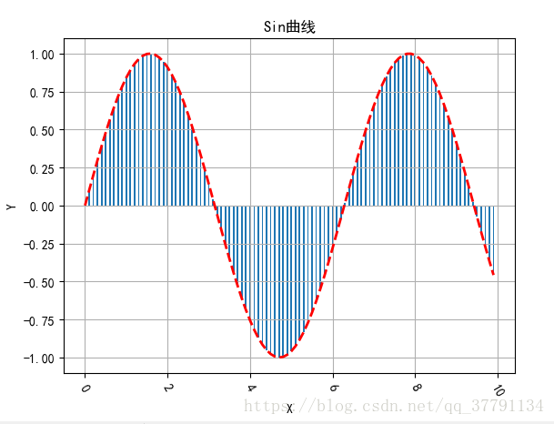
  # # 6.2 验证中心极限定理
    t = 1000
    a = np.zeros(10000)
    for i in range(t):
        a += np.random.uniform(-5, 5, 10000)
    a /= t
    plt.hist(a, bins=30, color='g', alpha=0.5, density=True, label=u'均匀分布叠加')
    plt.legend(loc='upper left')
    plt.grid(True, ls='--')
    plt.show()
中心极限定理用通俗的话来讲就是,假设有一个服从(μ,σ2)的总体,这个总体的分布可以是任意分布,不用是正态分布,既可以是离散的,也可以是连续的。我们从该分布里随机取n个样本x1,x2,...,xn,然后求这些样本的均值x_mean,这个过程我们重复m次,我们就会得到x_mean_1,x_mean_2,...,x_mean_m,如果n-->∞,这些样本的均值服从N(μ,σ2/n)的正态分布。
举例:我有1000个苹果,它们的重量服从μ=100,σ2=50的分布,每次从中随机的抽取5个苹果称重:
第一次选取的5个苹果的重量为:(89,78,101,22,150),均值x_mean_1=88
第二次。。。。。
。。。。
第m次选取的5个苹果的重量为:(77,90,34,88,140),均值x_mean_m=99.2
那这m次的样本的均值的分布为μ_mean = μ = 100, σ2_mean = σ2 / 5 = 50 / 5 = 10
--------------------- 本文来自 snowdroptulip 的CSDN 博客 ,全文地址请点击:https://blog.csdn.net/snowdroptulip/article/details/78969484?utm_source=copy
# # 6.2 验证中心极限定理
    t = 1000
    a = np.zeros(10000)
    for i in range(t):
        a += np.random.uniform(-3, 3, 10000)
    a /= t
    plt.hist(a, bins=30, color='g', alpha=0.5, density=True, label=u'均匀分布叠加')
    plt.legend(loc='upper left')
    plt.grid(True, ls='--')
    plt.show()
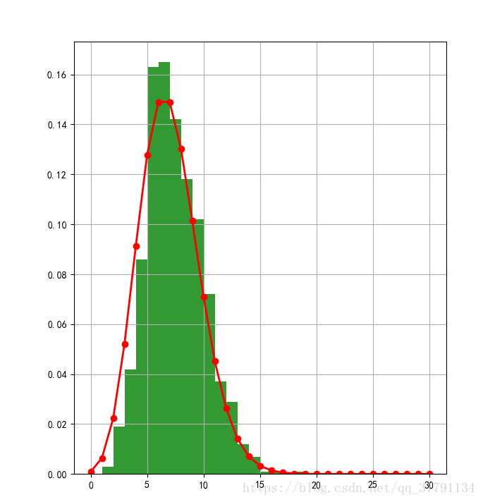
  # 6.21 其他分布的中心极限定理
    lamda = 7
    p = stats.poisson(lamda)
    y = p.rvs(size=1000)
    mx = 30
    r = (0, mx)
    bins = r[1] - r[0]
    plt.figure(figsize=(15, 8), facecolor='w')
    plt.subplot(121)
    plt.hist(y, bins=bins, range=r, color='g', alpha=0.8, normed=True)
    t = np.arange(0, mx+1)
    plt.plot(t, p.pmf(t), 'ro-', lw=2)
    plt.grid(True)
    N = 1000
    M = 10000
    plt.subplot(122)
    a = np.zeros(M, dtype=np.float)
    p = stats.poisson(lamda)
    for i in np.arange(N):
        a += p.rvs(size=M)
    a /= N
    plt.hist(a, bins=20, color='g', alpha=0.8, normed=True)
    plt.grid(b=True)
    plt.show()
  # 6.3 Poisson分布
    x = np.random.poisson(lam=5, size=10000)
    print(x)
    pillar = 15
    a = plt.hist(x, bins=pillar, density=True, range=[0, pillar], color='g', alpha=0.5)
    plt.grid()
    plt.show()
    print(a)
    print(a[0].sum())
    # # 6.4 直方图的使用
    mu = 2
    sigma = 3
    data = mu + sigma * np.random.randn(1000)
    h = plt.hist(data, 30, normed=1, color='#FFFFA0')
    x = h[1]
    y = norm.pdf(x, loc=mu, scale=sigma)
    plt.plot(x, y, 'r-', x, y, 'ro', linewidth=2, markersize=4)
    plt.grid()
    plt.show()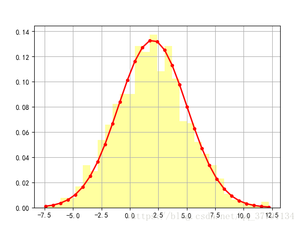
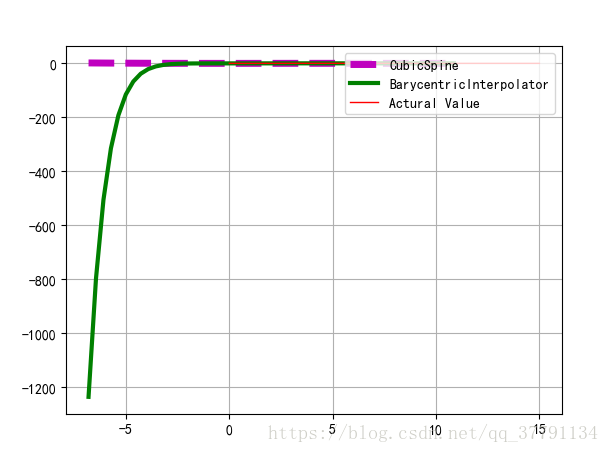
 # 6.5 插值
    rv = poisson(5)
    x1 = a[1]
    y1 = rv.pmf(x1)
    itp = BarycentricInterpolator(x1, y1)  # 重心插值
    x2 = np.linspace(x.min(), x.max(), 50)
    y2 = itp(x2)
    cs = sp.interpolate.CubicSpline(x1, y1)       # 三次样条插值
    plt.plot(x2, cs(x2), 'm--', linewidth=5, label='CubicSpine')           # 三次样条插值
    plt.plot(x2, y2, 'g-', linewidth=3, label='BarycentricInterpolator')   # 重心插值
    plt.plot(x1, y1, 'r-', linewidth=1, label='Actural Value')             # 原始值
    plt.legend(loc='upper right')
    plt.grid()
    plt.show()
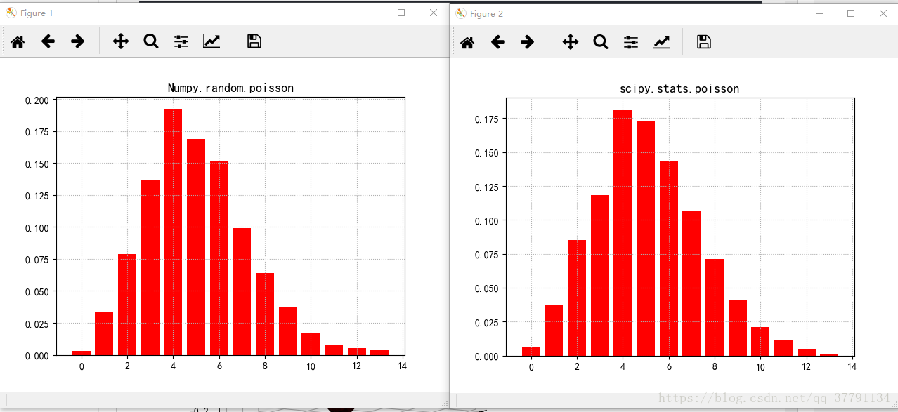
# 6.6 Poisson分布
    size = 1000
    lamda = 5
    p = np.random.poisson(lam=lamda, size=size)
    plt.figure()
    plt.hist(p, bins=range(3 * lamda), histtype='bar', align='left', color='r', rwidth=0.8, normed=True)
    plt.grid(b=True, ls=':')
    # plt.xticks(range(0, 15, 2))
    plt.title('Numpy.random.poisson', fontsize=13)

    plt.figure()
    r = stats.poisson(mu=lamda)
    p = r.rvs(size=size)
    plt.hist(p, bins=range(3 * lamda), color='r', align='left', rwidth=0.8, normed=True)
    plt.grid(b=True, ls=':')
    plt.title('scipy.stats.poisson', fontsize=13)
    plt.show()
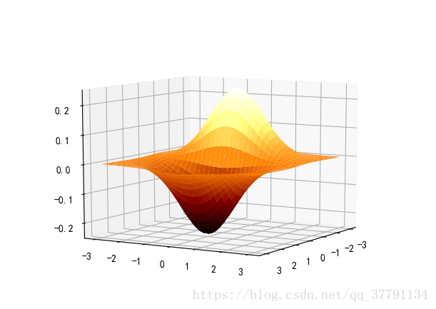
# 7. 绘制三维图像
    x, y = np.mgrid[-3:3:7j, -3:3:7j]
    print('x=', x)
    print('y=', y)
    u = np.linspace(-3, 3, 101)
    x, y = np.meshgrid(u, u)
    print('x =', x)
    print('y =', y)
    z = -x*np.exp(-(x**2 + y**2)/2) / math.sqrt(2*math.pi)
    # z = x*y*np.exp(-(x**2 + y**2)/2) / math.sqrt(2*math.pi)
    fig = plt.figure()
    ax = fig.add_subplot(111, projection='3d')
    # ax.plot_surface(x, y, z, rstride=5, cstride=5, cmap=cm.coolwarm, linewidth=0.1)  #
    ax.plot_surface(x, y, z, rstride=3, cstride=3, cmap=cm.afmhot, linewidth=0.5)
    plt.show()
    # # cmaps = [('Perceptually Uniform Sequential',
    # #           ['viridis', 'inferno', 'plasma', 'magma']),
    # #          ('Sequential', ['Blues', 'BuGn', 'BuPu',
    # #                          'GnBu', 'Greens', 'Greys', 'Oranges', 'OrRd',
    # #                          'PuBu', 'PuBuGn', 'PuRd', 'Purples', 'RdPu',
    # #                          'Reds', 'YlGn', 'YlGnBu', 'YlOrBr', 'YlOrRd']),
    # #          ('Sequential (2)', ['afmhot', 'autumn', 'bone', 'cool',
    # #                              'copper', 'gist_heat', 'gray', 'hot',
    # #                              'pink', 'spring', 'summer', 'winter']),
    # #          ('Diverging', ['BrBG', 'bwr', 'coolwarm', 'PiYG', 'PRGn', 'PuOr',
    # #                         'RdBu', 'RdGy', 'RdYlBu', 'RdYlGn', 'Spectral',
    # #                         'seismic']),
    # #          ('Qualitative', ['Accent', 'Dark2', 'Paired', 'Pastel1',
    # #                           'Pastel2', 'Set1', 'Set2', 'Set3']),
    # #          ('Miscellaneous', ['gist_earth', 'terrain', 'ocean', 'gist_stern',
    # #                             'brg', 'CMRmap', 'cubehelix',
    # #                             'gnuplot', 'gnuplot2', 'gist_ncar',
    # #                             'nipy_spectral', 'jet', 'rainbow',
    # #                             'gist_rainbow', 'hsv', 'flag', 'prism'])]
# 8.1 scipy
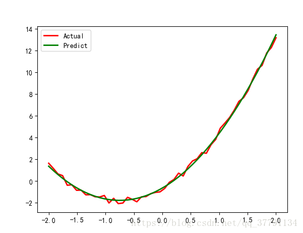
# 线性回归例1
x = np.linspace(-2, 2, 50)
A, B, C = 2, 3, -1
y = (A * x ** 2 + B * x + C) + np.random.rand(len(x))*0.75
t = leastsq(residual, [0, 0, 0], args=(x, y))
theta = t[0]
print('真实值:', A, B, C)
print('预测值:', theta)
y_hat = theta[0] * x ** 2 + theta[1] * x + theta[2]
plt.plot(x, y, 'r-', linewidth=2, label=u'Actual')
plt.plot(x, y_hat, 'g-', linewidth=2, label=u'Predict')
plt.legend(loc='upper left')
plt.grid()
plt.show()
 # # 线性回归例2
    x = np.linspace(0, 5, 100)
    a = 5
    w = 1.5
    phi = -2
    y = a * np.sin(w*x) + phi + np.random.rand(len(x))*0.5

    t = leastsq(residual2, [3, 5, 1], args=(x, y))
    theta = t[0]
    print('真实值:', a, w, phi)
    print('预测值:', theta)
    y_hat = theta[0] * np.sin(theta[1] * x) + theta[2]
    plt.plot(x, y, 'r-', linewidth=2, label='Actual')
    plt.plot(x, y_hat, 'g-', linewidth=2, label='Predict')
    plt.legend(loc='lower left')
    plt.grid()
    plt.show()
