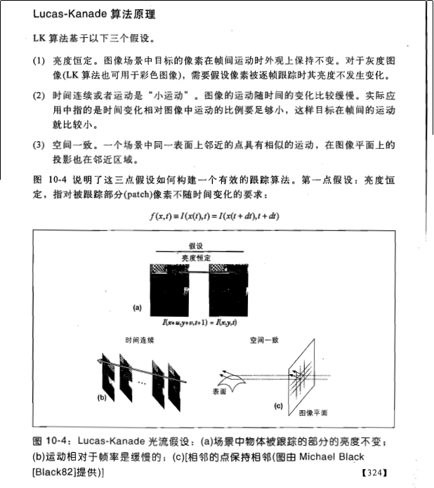
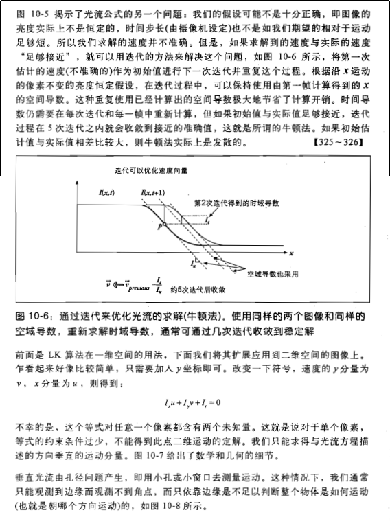
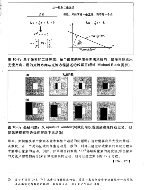
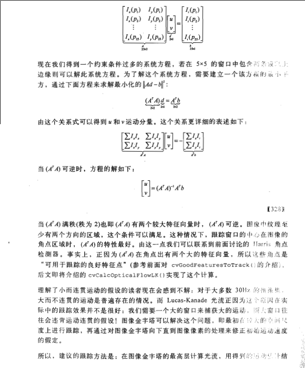
| 1 2 3 4 5 6 7 8 9 10 11 12 13 14 15 16 17 18 19 20 21 22 23 24 25 26 27 28 29 30 31 32 33 34 35 36 37 38 39 40 41 42 43 44 45 46 47 48 49 50 51 52 53 54 55 56 57 58 59 60 61 62 63 64 65 66 67 68 69 70 71 72 73 74 75 76 77 78 79 80 81 82 83 84 85 86 87 88 89 90 91 92 93 94 95 96 97 98 99 100 101 102 103 104 105 106 107 108 109 110 111 112 113 114 115 116 117 118 119 120 121 122 123 124 125 126 127 128 129 130 131 132 133 134 135 136 137 138 139 140 141 142 143 144 145 146 147 148 149 150 151 152 153 154 155 156 157 158 159 160 161 162 163 164 165 166 167 168 169 170 171 172 173 174 175 176 177 178 179 180 181 182 183 184 185 186 187 188 189 190 191 192 193 194 195 196 197 198 199 200 201 202 203 204 205 206 207 208 209 210 211 212 213 214 215 216 217 218 219 220 221 222 223 224 225 226 227 228 229 230 231 232 233 234 235 236 237 238 239 240 241 242 243 244 245 246 247 248 249 250 251 |
%%% Usage: Lucas_Kanade('1.bmp','2.bmp',10)
%%%%%%%%%%%%%%%%%%%%%%%%%%%%%%%%%%%%%%%%%%%%%%%%%%%%%%%%
%%%file1:输入图像1
%%%file2:输入图像2
%%%density:显示密度
function Lucas_Kanade(file1, file2, density)
%%% Read Images %% 读取图像
img1 = im2double (imread (file1));
%%% Take alternating rows and columns %% 按行分成奇偶
[odd1, ~] = split (img1);
img2 = im2double (imread (file2));
[odd2, ~] = split (img2);
%%% Run Lucas Kanade %% 运行光流估计
[Dx, Dy] = Estimate (odd1, odd2);
%%% Plot %% 绘图
figure;
[maxI,maxJ] = size(Dx);
Dx = Dx(1:density:maxI,1:density:maxJ);
Dy = Dy(1:density:maxI,1:density:maxJ);
quiver(1:density:maxJ, (maxI):(-density):1, Dx, -Dy, 1);
axis square;
%%% Run Lucas Kanade on all levels and interpolate %% 光流
function [Dx, Dy] = Estimate (img1, img2)
level = 4;%%%金字塔层数
half_window_size = 2;
% [m, n] = size (img1);
G00 = img1;
G10 = img2;
if (level > 0)%%%从零到level
G01 = reduce (G00); G11 = reduce (G10);
end
if (level>1)
G02 = reduce (G01); G12 = reduce (G11);
end
if (level>2)
G03 = reduce (G02); G13 = reduce (G12);
end
if (level>3)
G04 = reduce (G03); G14 = reduce (G13);
end
l = level;
for i = level: -1 :0,
if (l == level)
switch (l)
case 4, Dx = zeros (size (G04)); Dy = zeros (size (G04));
case 3, Dx = zeros (size (G03)); Dy = zeros (size (G03));
case 2, Dx = zeros (size (G02)); Dy = zeros (size (G02));
case 1, Dx = zeros (size (G01)); Dy = zeros (size (G01));
case 0, Dx = zeros (size (G00)); Dy = zeros (size (G00));
end
else
Dx = expand (Dx);
Dy = expand (Dy);
Dx = Dx .* 2;
Dy = Dy .* 2;
end
switch (l)
case 4,
W = warp (G04, Dx, Dy);
[Vx, Vy] = EstimateMotion (W, G14, half_window_size);
case 3,
W = warp (G03, Dx, Dy);
[Vx, Vy] = EstimateMotion (W, G13, half_window_size);
case 2,
W = warp (G02, Dx, Dy);
[Vx, Vy] = EstimateMotion (W, G12, half_window_size);
case 1,
W = warp (G01, Dx, Dy);
[Vx, Vy] = EstimateMotion (W, G11, half_window_size);
case 0,
W = warp (G00, Dx, Dy);
[Vx, Vy] = EstimateMotion (W, G10, half_window_size);
end
[m, n] = size (W);
Dx(1:m, 1:n) = Dx(1:m,1:n) + Vx; Dy(1:m, 1:n) = Dy(1:m, 1:n) + Vy;
smooth (Dx);
smooth (Dy);
l = l - 1;
end
%%% Lucas Kanade on the image sequence at pyramid step %%
function [Vx, Vy] = EstimateMotion (W, G1, half_window_size)
[m, n] = size (W);
Vx = zeros (size (W)); Vy = zeros (size (W));
N = zeros (2*half_window_size+1, 5);
for i = 1:m,
l = 0;
for j = 1-half_window_size:1+half_window_size,
l = l + 1;
N (l,:) = getSlice (W, G1, i, j, half_window_size);
end
replace = 1;
for j = 1:n,
t = sum (N);
[v, d] = eig ([t(1) t(2);t(2) t(3)]);
namda1 = d(1,1); namda2 = d(2,2);
if (namda1 > namda2)
tmp = namda1; namda1 = namda2; namda2 = tmp;
tmp1 = v (:,1); v(:,1) = v(:,2); v(:,2) = tmp1;
end
if (namda2 < 0.001)
Vx (i, j) = 0; Vy (i, j) = 0;
elseif (namda2 > 100 * namda1)
n2 = v(1,2) * t(4) + v(2,2) * t(5);
Vx (i,j) = n2 * v(1,2) / namda2;
Vy (i,j) = n2 * v(2,2) / namda2;
else
n1 = v(1,1) * t(4) + v(2,1) * t(5);
n2 = v(1,2) * t(4) + v(2,2) * t(5);
Vx (i,j) = n1 * v(1,1) / namda1 + n2 * v(1,2) / namda2;
Vy (i,j) = n1 * v(2,1) / namda1 + n2 * v(2,2) / namda2;
end
N (replace, :) = getSlice (W, G1, i, j+half_window_size+1, half_window_size);
replace = replace + 1;
if (replace == 2 * half_window_size + 2)
replace = 1;
end
end
end
%%% The Reduce Function for pyramid %%金字塔压缩
function result = reduce (ori)
[m,n] = size (ori);
mid = zeros (m, n);
%%%行列值的一半
m1 = round (m/2);
n1 = round (n/2);
%%%输出即为输入图像的1/4
result = zeros (m1, n1);
%%%滤波
%%%0.05 0.25 0.40 0.25 0.05
w = generateFilter (0.4);
for j = 1 : m,
tmp = conv([ori(j,n-1:n) ori(j,1:n) ori(j,1:2)], w);
mid(j,1:n1) = tmp(5:2:n+4);
end
for i=1:n1,
tmp = conv([mid(m-1:m,i); mid(1:m,i); mid(1:2,i)]', w);
result(1:m1,i) = tmp(5:2:m+4)';
end
%%% The Expansion Function for pyramid %%金字塔扩展
function result = expand (ori)
[m,n] = size (ori);
mid = zeros (m, n);
%%%行列值的两倍
m1 = m * 2;
n1 = n * 2;
%%%输出即为输入图像的4倍
result = zeros (m1, n1);
%%%滤波
%%%0.05 0.25 0.40 0.25 0.05
w = generateFilter (0.4);
for j=1:m,
t = zeros (1, n1);
t(1:2:n1-1) = ori (j,1:n);
tmp = conv ([ori(j,n) 0 t ori(j,1) 0], w);
mid(j,1:n1) = 2 .* tmp (5:n1+4);
end
for i=1:n1,
t = zeros (1, m1);
t(1:2:m1-1) = mid (1:m,i)';
tmp = conv([mid(m,i) 0 t mid(1,i) 0], w);
result(1:m1,i) = 2 .* tmp (5:m1+4)';
end
function filter = generateFilter (alpha)%%%滤波系数
filter = [0.25-alpha/2, 0.25, alpha, 0.25, 0.25-alpha/2];
function [N] = getSlice (W, G1, i, j, half_window_size)
N = zeros (1, 5);
[m, n] = size (W);
for y = -half_window_size:half_window_size,
Y1 = y +i;
if (Y1 < 1)
Y1 = Y1 + m;
elseif (Y1 > m)
Y1 = Y1 - m;
end
X1 = j;
if (X1 < 1)
X1 = X1 + n;
elseif (X1 > n)
X1 = X1 - n;
end
DeriX = Derivative (G1, X1, Y1, 'x'); %%%计算x、y方向梯度
DeriY = Derivative (G1, X1, Y1, 'y');
N = N + [ DeriX * DeriX, ...
DeriX * DeriY, ...
DeriY * DeriY, ...
DeriX * (G1 (Y1, X1) - W (Y1, X1)), ...
DeriY * (G1 (Y1, X1) - W (Y1, X1))];
end
function result = smooth (img)
result = expand (reduce (img));%%%太碉
function [odd, even] = split (img)
[m, ~] = size (img);%%%按行分成奇偶
odd = img (1:2:m, :);
even = img (2:2:m, :);
%%% Interpolation %% 插值
function result = warp (img, Dx, Dy)
[m, n] = size (img);
[x,y] = meshgrid (1:n, 1:m);
x = x + Dx (1:m, 1:n);
y = y + Dy (1:m,1:n);
for i=1:m,
for j=1:n,
if x(i,j)>n
x(i,j) = n;
end
if x(i,j)<1
x(i,j) = 1;
end
if y(i,j)>m
y(i,j) = m;
end
if y(i,j)<1
y(i,j) = 1;
end
end
end
result = interp2 (img, x, y, 'linear');%%%二维数据内插值
%%% Calculates the Fx Fy %% 计算x、y方向梯度
function result = Derivative (img, x, y, direction)
[m, n] = size (img);
switch (direction)
case 'x',
if (x == 1)
result = img (y, x+1) - img (y, x);
elseif (x == n)
result = img (y, x) - img (y, x-1);
else
result = 0.5 * (img (y, x+1) - img (y, x-1));
end
case 'y',
if (y == 1)
result = img (y+1, x) - img (y, x);
elseif (y == m)
result = img (y, x) - img (y-1, x);
else
result = 0.5 * (img (y+1, x) - img (y-1, x));
end
end
|

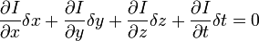
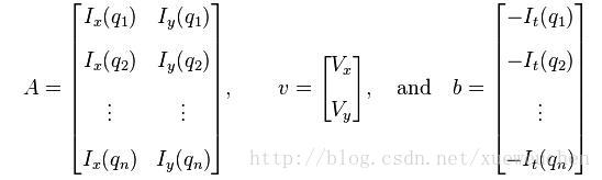
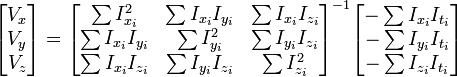
 ,
,  ,
,  和
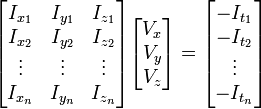
和  则是图像在(x ,y ,z ,t )这一点向相应方向的差分 。


 or
or
 来突出窗口中心点的坐标。高斯函数做这项工作是非常合适的,