什么是pytorch（3神经网络）(翻译)

神经网络

torch.nn 包可以用来构建神经网络。

前面介绍了 autograd包， nn 依赖于 autograd 用于定义和求导模型。 nn.Module 包括layers（神经网络层）, 以及forward函数 forward(input)，其返回结果 output.

例如我们来看一个手写数字的网络:

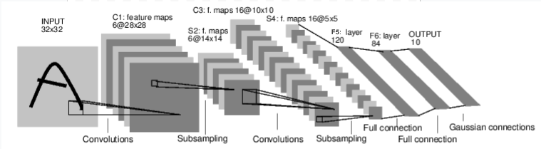
卷积神经网络

这是一个简单的前馈神经网络。接受输入，向前传几层，然后输出结果。

一个神经网络训练的简单过程是：

• 定义一个具有可学习参数的神经网络。
• 输入数据集迭代
• 网络运算数据输入的计算结果
• 计算损失 (how far is the output from being correct)
• 传播梯度
• 跟新权值，通常可以简单的使用梯度下降: weight = weight - learning_rate * gradient

定义网络

先来顶一个网络:

import torch
import torch.nn as nn import torch.nn.functional as F class Net(nn.Module): def __init__(self): super(Net, self).__init__() # 1 input image channel, 6 output channels, 5x5 square convolution # kernel self.conv1 = nn.Conv2d(1, 6, 5) self.conv2 = nn.Conv2d(6, 16, 5) # an affine operation: y = Wx + b self.fc1 = nn.Linear(16 * 5 * 5, 120) self.fc2 = nn.Linear(120, 84) self.fc3 = nn.Linear(84, 10) def forward(self, x): # Max pooling over a (2, 2) window x = F.max_pool2d(F.relu(self.conv1(x)), (2, 2)) # If the size is a square you can only specify a single number x = F.max_pool2d(F.relu(self.conv2(x)), 2) x = x.view(-1, self.num_flat_features(x)) x = F.relu(self.fc1(x)) x = F.relu(self.fc2(x)) x = self.fc3(x) return x def num_flat_features(self, x): size = x.size()[1:] # all dimensions except the batch dimension num_features = 1 for s in size: num_features *= s return num_features net = Net() print(net) 

Out:

Net(
  (conv1): Conv2d(1, 6, kernel_size=(5, 5), stride=(1, 1))
  (conv2): Conv2d(6, 16, kernel_size=(5, 5), stride=(1, 1))
  (fc1): Linear(in_features=400, out_features=120, bias=True)
  (fc2): Linear(in_features=120, out_features=84, bias=True)
  (fc3): Linear(in_features=84, out_features=10, bias=True)
)

你只需要定义前向传播函数 forward , 后向传播函数 backward (梯度的计算) 就会使用autograd自动定义。你可以在forward函数里使用任何Tensor的运算。

网络的学习到的参数可以通过net.parameters()获取。

params = list(net.parameters()) print(len(params)) print(params[0].size()) # conv1's .weight 

输出:

10
torch.Size([6, 1, 5, 5])

让我们随机输入一个 32x32 的数据。Note: Expected input size to this net(LeNet) is 32x32.

要把MNIST dataset作为该网络的数据集，需要把数据 resize到32x32.

input = torch.randn(1, 1, 32, 32) out = net(input) print(out) 

输出:

tensor([[ 0.1246, -0.0511,  0.0235,  0.1766, -0.0359, -0.0334,  0.1161,  0.0534,
          0.0282, -0.0202]], grad_fn=<ThAddmmBackward>)

使所有参数的梯度恢复为0，然后使用随机梯度后向传播:

net.zero_grad()
out.backward(torch.randn(1, 10)) 

注意：

torch.nn 只支持mini-batches. 整个 torch.nn 包只接受批样本，不接受单个样本。

例如, nn.Conv2d 接受一个4D的张量形如： nSamples x nChannels x Height x Width.

如果你只有一个样本，那就使用 input.unsqueeze(0) 创造一个假的mini-batch。

在进一步之前，我们来回顾目前你所见到的所有类。

回顾:

• torch.Tensor - 一个多维度的数组，支持自动梯度 backward()。其梯度任然保存在张量里。
• nn.Module - 神经网络模型。方便的封装参数，可以导出模型到GPU，加载模型，导出模型等。
• nn.Parameter - 一种张量, 自动注册为paramter当赋给 Module作为属性。
• autograd.Function - 实现 forward and backward 的定义，包括autograd. Every Tensor operation, creates at least a single Function node, that connects to functions that created a Tensor and encodes its history.

到此, 我们覆盖了:

• 定义一个网络
• 处理输入和反向传播。

剩余的内容:

• 计算损失
• 更新网络的参数

损失函数

一个损失函数接受（output,targe)对作为输入，计算output和target相差的程度。

nn包里有多种不同的 loss functions 。最简单的损失函数是: nn.MSELoss ，计算(output,target)间的均方误差损失函数。

For example:

output = net(input) target = torch.randn(10) # a dummy target, for example target = target.view(1, -1) # make it the same shape as output criterion = nn.MSELoss() loss = criterion(output, target) print(loss) 

输出:

tensor(1.3638, grad_fn=<MseLossBackward>)

Now, if you follow loss in the backward direction, using its .grad_fn attribute, you will see a graph of computations that looks like this:

input -> conv2d -> relu -> maxpool2d -> conv2d -> relu -> maxpool2d -> view -> linear -> relu -> linear -> relu -> linear -> MSELoss -> loss 

现在我们使用 loss.backward(),就会被 loss所微分, 所有计算图里参数属性为 requires_grad=True 将会使 .grad Tensor 和gradient累加起来。

For illustration, let us follow a few steps backward:

print(loss.grad_fn) # MSELoss print(loss.grad_fn.next_functions[0][0]) # Linear print(loss.grad_fn.next_functions[0][0].next_functions[0][0]) # ReLU 

Out:

<MseLossBackward object at 0x7f0e86396a90>
<ThAddmmBackward object at 0x7f0e863967b8>
<ExpandBackward object at 0x7f0e863967b8>

反向传播

为了反向传播误差，我们必须使用loss.backward(). 首先需要清除已存在的梯度，然后把梯度累加起来。

现在我们就可以调用：loss.backward(), 我们来看看 conv1’s bias gradients 在反向传播前后。

net.zero_grad()     # zeroes the gradient buffers of all parameters

print('conv1.bias.grad before backward') print(net.conv1.bias.grad) loss.backward() print('conv1.bias.grad after backward') print(net.conv1.bias.grad) 

输出:

conv1.bias.grad before backward
tensor([0., 0., 0., 0., 0., 0.])
conv1.bias.grad after backward
tensor([ 0.0181, -0.0048, -0.0229, -0.0138, -0.0088, -0.0107])

现在，我们来看如何使用损失函数。

进一步阅读:

nn包包括了各种类型的模型和损失函数，可以用来构建深度神经网络的block，详细参阅nn的文档： here.

最后一步需要学习的是:

• 跟新网络的参数

跟新权重Update the weights

最简单方式就是使用随机梯度下降（SGD):

weight = weight - learning_rate * gradient

可以使用以下代码:

learning_rate = 0.01
for f in net.parameters(): f.data.sub_(f.grad.data * learning_rate) 

神经网络里可以使用各种跟新权重的方法， 比如：SGD, Nesterov-SGD, Adam, RMSProp, etc等，为了使用这些方法，有一个小包 ： torch.optim 实现了这些方法。

用起来非常的容易：

import torch.optim as optim

# create your optimizer
optimizer = optim.SGD(net.parameters(), lr=0.01) # in your training loop: optimizer.zero_grad() # zero the gradient buffers output = net(input) loss = criterion(output, target) loss.backward() optimizer.step() # Does the update 

注意：

使用optimizer.zero_grad()把网络的参数梯度手动设置为0.前面在Backprop说了，梯度会累加起来的。