3.3.1均值文件mean file
数据预处理
transform_param
{
scale: 0.00390625
mean_file_size: “examples/cifar10/mean.binaryproto" #用一个配置文件来进行均值操作
mirror: 1
crop_size: 227
}
-
将所有训练样本的均值保存为文件
扫描二维码关注公众号,回复: 3391313 查看本文章
-
图片减去均值后,再进行训练和测试,会提高速度和精度】
-
运行方法:(使用caffe工具)
Compute_image_mean[train_lmdb][mean.binaryproto]
3.3.2 改写deploy 文件(以mnist为例)
-
把数据层(DATA Layer)和连接数据层的Layers 去掉(即top:data的层)
-
去掉输出层和连接输出层的Layers(即bottom:label)
-
重新建立输入
input:”data”
input_shape{
dim:1 #batchsize ,每次forward的时候输入的图片个数,这里1,就是,每次输入一张图片。
dim:3 #number of colour channels,1:灰度图,3:rgb图
dim:28 #width 和输入图片的格式大小保持一致。
dim:28#height
-
重新建立输出
| layer{ name:”prob” //与自己的网络名保持一致 type:”Softmax” bottom:”ip2” top:”prob” } |
修改后的mnist的deploy文件参考caffe/example/mnist/lenet.protxt
deploy.prototxt
| name: "LeNet" input: "data" //输入修改后的 input_shape { dim: 1 # batchsize dim: 1 # number of colour channels - rgb dim: 28 # width dim: 28 # height } layer { name: "conv1" type: "Convolution" bottom: "data" top: "conv1" param { lr_mult: 1 } param { lr_mult: 2 } convolution_param { num_output: 20 kernel_size: 5 stride: 1 weight_filler { type: "xavier" } bias_filler { type: "constant" } } } layer { name: "pool1" type: "Pooling" bottom: "conv1" top: "pool1" pooling_param { pool: MAX kernel_size: 2 stride: 2 } } layer { name: "conv2" type: "Convolution" bottom: "pool1" top: "conv2" param { lr_mult: 1 } param { lr_mult: 2 } convolution_param { num_output: 50 kernel_size: 5 stride: 1 weight_filler { type: "xavier" } bias_filler { type: "constant" } } } layer { name: "pool2" type: "Pooling" bottom: "conv2" top: "pool2" pooling_param { pool: MAX kernel_size: 2 stride: 2 } } layer { name: "ip1" type: "InnerProduct" bottom: "pool2" top: "ip1" param { lr_mult: 1 } param { lr_mult: 2 } inner_product_param { num_output: 500 weight_filler { type: "xavier" } bias_filler { type: "constant" } } } layer { name: "relu1" type: "ReLU" bottom: "ip1" top: "ip1" } layer { name: "ip2" type: "InnerProduct" bottom: "ip1" top: "ip2" param { lr_mult: 1 } param { lr_mult: 2 } inner_product_param { num_output: 10 weight_filler { type: "xavier" } bias_filler { type: "constant" } } } layer { //修改后的输出 name: "prob" type: "Softmax" bottom: "ip2" top: "prob" } |
3.3.3 实操演示:训练自己的模型
1、数据准备
推荐官网:http://www.image-net.org/download-images
下载地址:http://pan.baidu.com/s/1nuqlTnN
数据集:500张、分5类、每类100张,编号分别以3,4,5,6,7开头,各为一类。每类选出20张作为测试,其余80张作为训练。
数据集存放地址:caffe/data 训练图片目录:data/re/train/ ,测试图片目录: data/re/test/
-
转换为lmdb格式
#caffe目录下
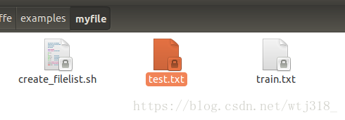
#在examples下面创建一个myfile文件夹,来存放配置文件和脚本文件
#编写一个脚本create_filelist.sh,用来生成train.txt和test.txt
$mkdir examples/myfile
$sudo vi examples/myfile/create_filelist.sh
#编辑
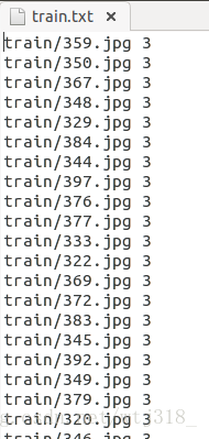
| #!/usr/bin/env sh DATA=data/re/ //数据目录 MY=examples/myfile //脚本目录 echo "Create train.txt..." rm -rf $MY/train.txt //重复建立错误排除 for i in 3 4 5 6 7 //以图片名称首字母分类 do find $DATA/train -name $i*.jpg | cut -d '/' -f4-5 | sed "s/$/ $i/">>$MY/train.txt //在图片列表行最前面加上train属性,最后加上该图片首字母的标签,即分类列表 done echo "Create test.txt..." rm -rf $MY/test.txt for i in 3 4 5 6 7 do find $DATA/test -name $i*.jpg | cut -d '/' -f4-5 | sed "s/$/ $i/">>$MY/test.txt done echo "All done" |
#运行脚本,生成图片列表
$sudo sh examples/myfile/create_filelist.sh
#再编写脚本,调用convert_imageset命令来转换数据格式
$sudo vi examples/myfile/create_lmdb.sh
#编辑
| #!/bin/bash #!/usr/bin/env sh MY=examples/myfile echo "Create train lmdb.." rm -rf $MY/img_train_lmdb build/tools/convert_imageset \ --shuffle \ --resize_height=256 \ --resize_width=256 \ /home/wtj/caffe/data/re/ \ $MY/train.txt \ $MY/img_train_lmdb echo "Create test lmdb.." rm -rf $MY/img_test_lmdb build/tools/convert_imageset \ --shuffle \ --resize_width=256 \ --resize_height=256 \ /home/wtj/caffe/data/re/ \ $MY/test.txt \ $MY/img_test_lmdb echo "All Done.." |
$sudo sh examples/myfile/create_lmdb.sh

#生成train和test lmdb 数据

-
计算均值并保存
图片减去均值后再训练,会提高训练速度和精度,因此,一般都会有此操作。
Caffe程序提供了一个计算均值的文件compute_image_mean.cpp,可直接使用
$ sudo build/tools/compute_image_mean examples/myfile/img_train_lmdb
examples/myfile/mean.binaryproto
#compute_image_mean带两个参数,第一个参数是lmdb训练数据位置,第二个参数设定均值文件的名字
#及保存路径。运行成功后,会在 examples/myfile/ 下面生成一个mean.binaryproto的均值文件。

-
创建模型并编写配置文件
模型就用程序自带的caffenet模型,位置在 models/bvlc_reference_caffenet/文件夹下, 将需要的两个配置文件,复制到myfile文件夹内
$ sudo cp models/bvlc_reference_caffenet/solver.prototxt examples/myfile
$ sudo cp models/bvlc_reference_caffenet/train_val.prototxt examples/myfile/
#修改solver.prototxt
$sudo vi examples/myfile/solver.prototxt
#编辑
| net: "examples/myfile/train_val.prototxt" test_iter: 2 //100个测试集,batchsize:50,所以test_iter:2 test_interval: 50 base_lr: 0.001 lr_policy: "step" gamma: 0.1 stepsize: 100 display: 20 max_iter: 500 momentum: 0.9 weight_decay: 0.005 solver_mode: CPU |
#修改train_val.protxt,只需要修改两个阶段的data层就可以了,其它可以不用管。
$sudo vi examples/myfile/train_val.protxt
#编辑,只需要修改两个阶段的data层就可以,其他不用管。
| name: "CaffeNet" layer { name: "data" type: "Data" top: "data" top: "label" include { phase: TRAIN } transform_param { mirror: true crop_size: 227 mean_file: "examples/myfile/mean.binaryproto" } data_param { source: "examples/myfile/img_train_lmdb" batch_size: 256 backend: LMDB } } layer { name: "data" type: "Data" top: "data" top: "label" include { phase: TEST } transform_param { mirror: false crop_size: 227 mean_file: "examples/myfile/mean.binaryproto" } data_param { source: "examples/myfile/img_test_lmdb" batch_size: 50 backend: LMDB } } |
实际上就是修改两个data layer的mean_file和source这两个地方,其它都没有变化
-
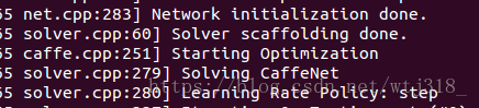
训练和测试
$ sudo build/tools/caffe train -solver examples/myfile/solver.prototxt
#开始建楼
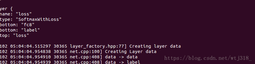
#统计内存占用情况
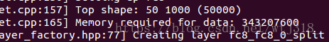
#盖最后一层loss
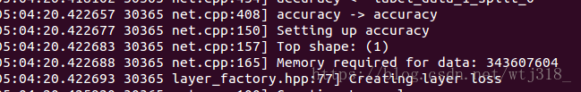
#loss尺寸:1,loss weight:1
#开始装修
#测试第一次
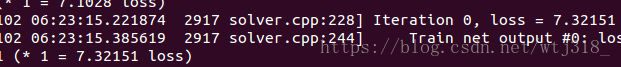
#
3.3.4 使用fine turning微调网络
1. 准备新数据的数据库(如果需要用mean file,还要准备对应的新的mean file), 具体方法和图片转换lmdb方式一样。
2. 调整网络层参数:
将来训练的网络配置prototxt中的数据层source换成新数据的数据库。
调整学习率,因为最后一层是重新学习,因此需要有更快的学习速率相比较其他层,因此我们将,weight和bias的学习速率加快。
3. 修改solver参数
原来的数据是从原始数据开始训练的,因此一般来说学习速率、步长、迭代次数都比较大,fine turning微调时,因为数据量可能减少了,所以一般来说,test_iter,base_lr,stepsize都要变小一点,其他的策略可以保持不变。
4. 重新训练时,要指定之前的权值文件:
# caffe train --solver [新的solver文件] --weights [旧的caffemodel]