【123】TensorFlow 多个特征值线性回归，并且使用训练集、验证集和测试集的例子

版权声明：本文为博主原创文章，未经博主允许不得转载。 https://blog.csdn.net/zhangchao19890805/article/details/82422333

我使用加利福尼亚州房价数据来作例子。训练集和验证集用到的CSV文件在这里：https://download.csdn.net/download/zhangchao19890805/10584496

测试集用到的CSV文件在这里： https://download.csdn.net/download/zhangchao19890805/10631336

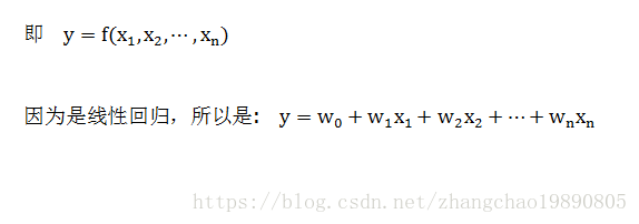
我们的目标是构建数学模型来预测房价。通常情况下，会有多个因素影响房价，因此使用多个特征值做线性回归。数学上，每个特征值视为一个自变量，相当与构建一个包含多个自变量的函数。

我写了两个 python 文件，一个是用来训练模型，并使用验证集验证模型。另一个是用测试集测试我的数学模型。

在程序中，使用到的特征值是这些：latitude、 longitude、
housing_median_age、total_rooms、 total_bedrooms、population、 households、 median_income 和 rooms_per_person

训练模型的文件：

import tensorflow as tf
import numpy as np
import matplotlib.pyplot as plt
import pandas as pd
import math
from sklearn import metrics

# 从CSV文件中读取数据，返回DataFrame类型的数据集合。
def zc_func_read_csv():
    zc_var_dataframe = pd.read_csv("http://114.115.223.20/california_housing_train.csv", sep=",")
    # 打乱数据集合的顺序。有时候数据文件有可能是根据某种顺序排列的，会影响到我们对数据的处理。
    zc_var_dataframe = zc_var_dataframe.reindex(np.random.permutation(zc_var_dataframe.index))
    return zc_var_dataframe

# 预处理特征值
def preprocess_features(california_housing_dataframe):
    selected_features = california_housing_dataframe[
        ["latitude",
         "longitude",
         "housing_median_age",
         "total_rooms",
         "total_bedrooms",
         "population",
         "households",
         "median_income"]
    ]
    processed_features = selected_features.copy()
    # 增加一个新属性：人均房屋数量。
    processed_features["rooms_per_person"] = (
        california_housing_dataframe["total_rooms"] /
        california_housing_dataframe["population"])
    return processed_features

# 预处理标签
def preprocess_targets(california_housing_dataframe):
    output_targets = pd.DataFrame()
    # Scale the target to be in units of thousands of dollars.
    output_targets["median_house_value"] = (
        california_housing_dataframe["median_house_value"] / 1000.0)
    return output_targets

def zc_func_yhat_eval(zc_param_yhat):
    r = []
    for ele in zc_param_yhat:
        r.append(ele[0])
    return r

# 根据数学模型计算预测值。公式是 y = w0 + w1 * x1 + w2 * x2 .... + w9 * x9
def zc_func_predict(zc_param_dataframe, zc_param_weight_arr):
    zc_var_result = []
    for var_row_index in zc_param_dataframe.index:
        y = zc_param_weight_arr[0]
        y = y + zc_param_weight_arr[1] * zc_param_dataframe.loc[var_row_index].values[0]
        y = y + zc_param_weight_arr[2] * zc_param_dataframe.loc[var_row_index].values[1]
        y = y + zc_param_weight_arr[3] * zc_param_dataframe.loc[var_row_index].values[2]
        y = y + zc_param_weight_arr[4] * zc_param_dataframe.loc[var_row_index].values[3]
        y = y + zc_param_weight_arr[5] * zc_param_dataframe.loc[var_row_index].values[4]
        y = y + zc_param_weight_arr[6] * zc_param_dataframe.loc[var_row_index].values[5]
        y = y + zc_param_weight_arr[7] * zc_param_dataframe.loc[var_row_index].values[6]
        y = y + zc_param_weight_arr[8] * zc_param_dataframe.loc[var_row_index].values[7]
        y = y + zc_param_weight_arr[9] * zc_param_dataframe.loc[var_row_index].values[8]
        zc_var_result.append(y)
    return zc_var_result



# 训练形如 y = w0 + w1 * x1 + w2 * x2 + ...  的直线模型。x1 x2 ...是自变量，
# w0 是常数项，w1 w2 ... 是对应自变量的权重。
# feature_arr 特征值的矩阵。每一行是 [1.0, x1_data, x2_data, ...] 
# label_arr 标签的数组。相当于 y = kx + b 中的y。
# training_steps 训练的步数。即训练的迭代次数。
# period         误差报告粒度
# learning_rate 在梯度下降算法中，控制梯度步长的大小。
def zc_fn_train_line(feature_arr, label_arr, validate_feature_arr, validate_label_arr, training_steps, periods, learning_rate):
    feature_tf_arr = feature_arr
    label_tf_arr = np.array([[e] for e in label_arr]).astype(np.float32)
    # 整个训练分成若干段，即误差报告粒度，用periods表示。
    # steps_per_period 表示平均每段有多少次训练
    steps_per_period = training_steps / periods
    # 存放 L2 损失的数组
    loss_arr = []
    weight_arr_length = len(feature_arr[0])
    # 开启TF会话，在TF 会话的上下文中进行 TF 的操作。
    with tf.Session() as sess:
        # 训练集的均方根误差RMSE。这是保存误差报告的数组。
        train_rmse_arr = []
        # 验证集的均方根误差RMSE。
        validate_rmse_arr = []

        # 设置 tf 张量（tensor）。注意：TF会话中的注释里面提到的常量和变量是针对TF设置而言，不是python语法。

        # 因为在TF运算过程中，x作为特征值，y作为标签
        # 是不会改变的，所以分别设置成input 和 target 两个常量。
        # 这是 x 取值的张量。设一共有m条数据，可以把input理解成是一个m行2列的矩阵。矩阵第一列都是1，第二列是x取值。
        input = tf.constant(feature_tf_arr)
        # 设置 y 取值的张量。target可以被理解成是一个m行1列的矩阵。 有些文章称target为标签。
        target = tf.constant(label_tf_arr)

        # 设置权重变量。因为在每次训练中，都要改变权重，来寻找L2损失最小的权重，所以权重是变量。
        # 可以把权重理解成一个多行1列的矩阵。初始值是随机的。行数就是权重数。
        weights = tf.Variable(tf.random_normal([weight_arr_length, 1], 0, 0.1))

        # 初始化上面所有的 TF 常量和变量。
        tf.global_variables_initializer().run()
        # input 作为特征值和权重做矩阵乘法。m行2列矩阵乘以2行1列矩阵，得到m行1列矩阵。
        # yhat是新矩阵，yhat中的每个数 yhat' = w0 * 1 + w1 * x1 + w2 * x2 ...。 
        # yhat是预测值，随着每次TF调整权重，yhat都会变化。
        yhat = tf.matmul(input, weights)
        # tf.subtract计算两个张量相减，当然两个张量必须形状一样。 即 yhat - target。
        yerror = tf.subtract(yhat, target)
        # 计算L2损失，也就是方差。
        loss = tf.nn.l2_loss(yerror)
        # 梯度下降算法。
        zc_optimizer = tf.train.GradientDescentOptimizer(learning_rate)
        # 注意：为了安全起见，我们还会通过 clip_gradients_by_norm 将梯度裁剪应用到我们的优化器。
        # 梯度裁剪可确保梯度大小在训练期间不会变得过大，梯度过大会导致梯度下降法失败。
        zc_optimizer = tf.contrib.estimator.clip_gradients_by_norm(zc_optimizer, 5.0)
        zc_optimizer = zc_optimizer.minimize(loss)
        for _ in range(periods):
            for _ in range(steps_per_period):
                # 重复执行梯度下降算法，更新权重数值，找到最合适的权重数值。
                sess.run(zc_optimizer)
                # 每次循环都记录下损失loss的值，并放到数组loss_arr中。
                loss_arr.append(loss.eval())
            v_tmp_weight_arr = weights.eval()
            train_rmse_arr.append(math.sqrt(
                    metrics.mean_squared_error(zc_func_yhat_eval(yhat.eval()), label_tf_arr)))
            validate_rmse_arr.append(math.sqrt(
                    metrics.mean_squared_error(zc_func_predict(validate_feature_arr, v_tmp_weight_arr), validate_label_arr)))
        zc_weight_arr = weights.eval()
        zc_yhat = yhat.eval()
    return (zc_weight_arr, zc_yhat, loss_arr, train_rmse_arr, validate_rmse_arr)
# end def train_line


# 构建用于训练的特征值。
# zc_var_dataframe 原来数据的 Dataframe
# 本质上是用二维数组构建一个矩阵。里面的每个一维数组都是矩阵的一行，形状类似下面这种形式：
#    1.0, x1[0], x2[0], x3[0], ...
#    1.0, x1[1], x2[1], x3[1], ...
#    .........................
# 其中x1, x2, x3 表示数据的某个维度，比如："latitude","longitude","housing_median_age"。
# 也可以看作是公式中的多个自变量。
def zc_func_construct_tf_feature_arr(zc_var_dataframe):
    zc_var_result = []
    # dataframe中每列的名称。
    zc_var_col_name_arr = [e for e in zc_var_dataframe]
    # 遍历dataframe中的每行。
    for row_index in zc_var_dataframe.index:
        zc_var_tf_row = [1.0]
        for i in range(len(zc_var_col_name_arr)):
            zc_var_tf_row.append(zc_var_dataframe.loc[row_index].values[i])
        zc_var_result.append(zc_var_tf_row)
    return zc_var_result

# 画损失的变化图。
# ax  Axes
# zc_param_learning_steps 训练次数。
# zc_param_loss_arr 每次训练，损失变化的记录
def zc_func_paint_loss(ax, arr_train_rmse, arr_validate_rmse):
    ax.plot(range(0, len(arr_train_rmse)), arr_train_rmse, label="training", color="blue")
    ax.plot(range(0, len(arr_validate_rmse)), arr_validate_rmse, label="validate", color="orange")

# 主函数 
def zc_func_main():

    california_housing_dataframe = zc_func_read_csv()
    # 对于训练集，我们从共 17000 个样本中选择前 12000 个样本。
    training_examples = preprocess_features(california_housing_dataframe.head(12000))
    training_targets = preprocess_targets(california_housing_dataframe.head(12000))
    # 对于验证集，我们从共 17000 个样本中选择后 5000 个样本。
    validation_examples = preprocess_features(california_housing_dataframe.tail(5000))
    validation_targets = preprocess_targets(california_housing_dataframe.tail(5000))

    fig = plt.figure()
    fig.set_size_inches(5,5)


    zc_var_train_feature_arr = zc_func_construct_tf_feature_arr(training_examples)
    zc_var_leaning_step_num = 500
    (zc_weight_arr, zc_yhat, loss_arr, train_rmse_arr, validate_rmse_arr) = zc_fn_train_line(zc_var_train_feature_arr, 
                    training_targets["median_house_value"], validation_examples, 
                    validation_targets["median_house_value"], zc_var_leaning_step_num, 20, 0.002)
    # 画损失变化图。
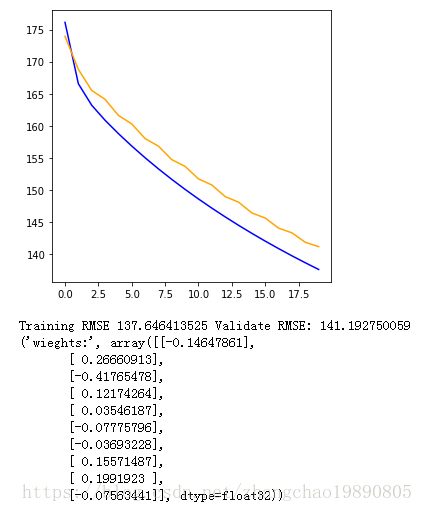
    zc_func_paint_loss(fig.add_subplot(1,1,1), train_rmse_arr, validate_rmse_arr)
    plt.show()

    print("Training RMSE " + str(train_rmse_arr[len(train_rmse_arr) - 1]) + " Validate RMSE: " + 
          str(validate_rmse_arr[len(validate_rmse_arr) - 1]))

    print("wieghts:", zc_weight_arr)



zc_func_main()

运行结果如下

然后我们用测试集来测试模型：

import tensorflow as tf
import numpy as np
import matplotlib.pyplot as plt
import pandas as pd
import math
from sklearn import metrics


# 从CSV文件中读取数据，返回DataFrame类型的数据集合。
def zc_func_read_csv(zc_param_csv_url):
#     zc_var_dataframe = pd.read_csv("http://49.4.2.82/california_housing_train.csv", sep=",")
    zc_var_dataframe = pd.read_csv(zc_param_csv_url, sep=",")
    # 打乱数据集合的顺序。有时候数据文件有可能是根据某种顺序排列的，会影响到我们对数据的处理。
    zc_var_dataframe = zc_var_dataframe.reindex(np.random.permutation(zc_var_dataframe.index))
    return zc_var_dataframe

# 预处理特征值
def preprocess_features(california_housing_dataframe):
    selected_features = california_housing_dataframe[
        ["latitude",
         "longitude",
         "housing_median_age",
         "total_rooms",
         "total_bedrooms",
         "population",
         "households",
         "median_income"]
    ]
    processed_features = selected_features.copy()
    # 增加一个新属性：人均房屋数量。
    processed_features["rooms_per_person"] = (
        california_housing_dataframe["total_rooms"] /
        california_housing_dataframe["population"])
    return processed_features

# 预处理标签
def preprocess_targets(california_housing_dataframe):
    output_targets = pd.DataFrame()
    # Scale the target to be in units of thousands of dollars.
    output_targets["median_house_value"] = (
        california_housing_dataframe["median_house_value"] / 1000.0)
    return output_targets


# 根据数学模型计算预测值。公式是 y = w0 + w1 * x1 + w2 * x2 .... + w9 * x9
def zc_func_predict(zc_param_dataframe, zc_param_weight_arr):
    zc_var_result = []
    for var_row_index in zc_param_dataframe.index:
        y = zc_param_weight_arr[0]
        y = y + zc_param_weight_arr[1] * zc_param_dataframe.loc[var_row_index].values[0]
        y = y + zc_param_weight_arr[2] * zc_param_dataframe.loc[var_row_index].values[1]
        y = y + zc_param_weight_arr[3] * zc_param_dataframe.loc[var_row_index].values[2]
        y = y + zc_param_weight_arr[4] * zc_param_dataframe.loc[var_row_index].values[3]
        y = y + zc_param_weight_arr[5] * zc_param_dataframe.loc[var_row_index].values[4]
        y = y + zc_param_weight_arr[6] * zc_param_dataframe.loc[var_row_index].values[5]
        y = y + zc_param_weight_arr[7] * zc_param_dataframe.loc[var_row_index].values[6]
        y = y + zc_param_weight_arr[8] * zc_param_dataframe.loc[var_row_index].values[7]
        y = y + zc_param_weight_arr[9] * zc_param_dataframe.loc[var_row_index].values[8]
        zc_var_result.append(y)

    return zc_var_result


def zc_func_main():
    california_housing_dataframe = zc_func_read_csv("http://114.115.223.20/california_housing_train.csv")
    # 对于验证集，我们从共 17000 个样本中选择后 5000 个样本。
    validation_examples = preprocess_features(california_housing_dataframe.tail(5000))
    #print(validation_examples.describe())
    validation_targets = preprocess_targets(california_housing_dataframe.tail(5000))
    # 通过训练得到的模型权重
    zc_param_weight_arr = [-0.19103946,0.37296584,-0.7998271,0.25258455,0.03940793,-0.13476478,
                           -0.04755316,0.20973271,0.00714895,0.02928887]
    # 根据已经训练得到的模型系数，计算预验证集的测值。
    zc_var_validate_predict_arr = zc_func_predict(validation_examples, zc_param_weight_arr)
    # 计算验证集的预测值和标签之间的均方根误差。
    validation_root_mean_squared_error = math.sqrt(
        metrics.mean_squared_error(zc_var_validate_predict_arr, validation_targets["median_house_value"]))
    print("validation RMSE:", validation_root_mean_squared_error)


    # 基于测试集数据进行评估
    test_dataframe = zc_func_read_csv("http://114.115.223.20/california_housing_test.csv")
    # 测试集的样本
    test_examples = preprocess_features(test_dataframe)
    test_targets = preprocess_targets(test_dataframe)
    # 计算测试集的预测值
    zc_var_test_predict_arr = zc_func_predict(test_examples, zc_param_weight_arr)
    # 计算测试集的预测值和标签之间的均方根误差。
    test_root_mean_squared_error = math.sqrt(
        metrics.mean_squared_error(zc_var_test_predict_arr, test_targets["median_house_value"]))
    print("test RMSE:", test_root_mean_squared_error)

zc_func_main()

运行结果：

('validation RMSE:', 120.00240785178423)
('test RMSE:', 116.6171534701997)