节选自《Machine Learning in Action》——Peter Harrington
中文版是《机器学习实战》
本文介绍的是ID3算法,用python实现,编译器为jupyter
优点:计算复杂度不高,输出结果易于理解,对中间值的缺失不敏感,可以处理不相关特征数据
缺点:可能会产生过度匹配的问题
决策树的一般流程
- 收集数据:anyway
- 准备数据:离散化
- 分析数据:anyway,构造数完成后,检查树是否符合预期
- 训练算法:构造树的数据结构
- 测试算法:使用经验树计算错误率
- 使用算法:适用于任何监督学习算法,而使用决策树可以更好的理解数据的内在含义
1 决策树的构造
1.1 信息增益
实验数据集如下:

构建数据集函数
# trees.py(1) 第一段代码,初始化数据集
from math import log
import operator
# 构建数据集
def createDataSet():
    dataSet = [[1, 1, 'yes'],
               [1, 1, 'yes'],
               [1, 0, 'no'],
               [0, 1, 'no'],
               [0, 1, 'no']]
    labels = ['no surfacing','flippers']#没露出水面,脚蹼
    #change to discrete values
    return dataSet, labels
调用一下
from math import log
import trees #决策树代码,trees.py
import operator
#调用createDataSet()
myDat,labels = trees.createDataSet()
print ('myDat:',myDat)
print ('labels:',labels)
结果为
myDat: [[1, 1, 'yes'], [1, 1, 'yes'], [1, 0, 'no'], [0, 1, 'no'], [0, 1, 'no']]
labels: ['no surfacing', 'flippers']
计算信息增益
克劳德·香农写完信息论后,约翰·冯·诺依曼建议使用“熵”这个术语。“贝尔实验室和MIT有很多人将香农和爱因斯坦相提并论,而其他人则认为这种对比是不公平的——对香农是不公平的”
如果待分类的事务可能划分在多个分类之中,则某一类
的信息定义如下:
其中 是选择分类的概率
为了计算熵,我们需要计算所有类别所有可能包含的信息期望值,通过下面公式得到:
Note:熵值越高,系统越杂乱,混合的数据也越多!可以这样理解,事物总是趋向于混乱,也就是熵增。越纯,p越接近于1,log越接近于0,熵也就越小。
# trees.py(2) 第2段代码,计算样本的熵值
def calcShannonEnt(dataSet):
    numEntries = len(dataSet) # 5
    labelCounts = {} #为所有可能分类创建字典
    for featVec in dataSet: #[1, 1, 'yes'],[1, 1, 'yes']
        currentLabel = featVec[-1] #第一个样本的labes,eg: yes, no
        if currentLabel not in labelCounts.keys():
            labelCounts[currentLabel] = 0
        labelCounts[currentLabel] += 1
    #labelCounts is {'yes': 2, 'no': 3}
    shannonEnt = 0.0
    for key in labelCounts:# key is yes or no
        prob = float(labelCounts[key])/numEntries #计算概率p,当前label的数量除以label的总数量
        shannonEnt -= prob * log(prob,2) #log base 2
    return shannonEnt
测试下
trees.calcShannonEnt(myDat)结果为
0.9709505944546686增加新的一类
myDat[0][-1]='maybe'#第一组最后一个属性,改为maybe
trees.calcShannonEnt(myDat)
结果为
1.3709505944546687说明:熵值越高,系统越杂乱,混合的数据也越多
1.2 划分数据集
# trees.py(3) 第3段代码,按给定特征划分数据集
#第axis列选出来,与value对比,相等,输出除axis的列
def splitDataSet(dataSet, axis, value):
    retDataSet = []
    for featVec in dataSet: # featVec is [1, 1, 'yes'],[1, 1, 'yes']
        if featVec[axis] == value:
            reducedFeatVec = featVec[:axis]     #chop out axis used for splitting,[0,axis)
            reducedFeatVec.extend(featVec[axis+1:])#[axis+1,last)
            retDataSet.append(reducedFeatVec)
    return retDataSet
测试下
myDat,labels = trees.createDataSet()
# DataSet,axis,val
print (trees.splitDataSet(myDat,0,1)) #第axis列选出来,与value对比,相等,输出除axis的列
print (trees.splitDataSet(myDat,0,0))
print (trees.splitDataSet(myDat,1,0))
结果
[[1, 'yes'], [1, 'yes'], [0, 'no']]
[[1, 'no'], [1, 'no']]
[[1, 'no']]
有了划分数据集的方法还不够,我们要选择最好的数据划分方式,思路为
遍历所有特征,统计每个特征下的属性种类,按照属性,调用数据划分函数划分数据集,然后计算划分后的熵,保留熵值最大的特征,作为bestFeature,注意输出结果是特征的序号,0代表第一个特征,1代表第二个特征。
具体实现如下:
# trees.py(4) 第4段代码,选择最好的数据集划分方式
def chooseBestFeatureToSplit(dataSet):
    numFeatures = len(dataSet[0]) - 1      #the last column is used for the labels,2
    baseEntropy = calcShannonEnt(dataSet) #0.9709505944546686
    bestInfoGain = 0.0; bestFeature = -1
    for i in range(numFeatures):        #iterate over all the features
        featList = [example[i] for example in dataSet]#create a list of all the examples of this feature
        # 第一次循环为[1, 1, 1, 0, 0],五个样本的第一个特征
        uniqueVals = set(featList)       #get a set of unique values,变成了一个集合,{0,1}
        newEntropy = 0.0
        for value in uniqueVals:
            subDataSet = splitDataSet(dataSet, i, value)#第i列特征值,与value比较,算出信息熵
            prob = len(subDataSet)/float(len(dataSet))
            newEntropy += prob * calcShannonEnt(subDataSet)
        infoGain = baseEntropy - newEntropy     #calculate the info gain; ie reduction in entropy
        #这个位置注意了,划分数据后,数据更有序,数据entropy变小了
        #0.4199730940219749 , 0.17095059445466854
        if (infoGain > bestInfoGain):       #compare this to the best gain so far
            bestInfoGain = infoGain         #if better than current best, set to best
            bestFeature = i
    return bestFeature                     #returns an integer
测试一下
trees.chooseBestFeatureToSplit(myDat)结果为
01.3 递归构建决策树
有选取最优特征的方法后,我们就可以递归的构造决策树
递归结束的条件是
1. 程序遍历完所有划分数据集的属性,或者
2. 每个分支下的所有实例都具有相同的分类
上述第一种情况发生后,如果类标签依旧不是唯一的,此时我们需要决定如何定义该叶子节点,在这种情况下,我们通常会采用多数表决的方法决定该叶子节点的分类
# trees.py(5) 第5段代码,投票机制
def majorityCnt(classList):
    classCount={}
    for vote in classList:
        if vote not in classCount.keys(): classCount[vote] = 0
        classCount[vote] += 1
    sortedClassCount = sorted(classCount.items(), key=operator.itemgetter(1), reverse=True)
    # reverse = True 默认降序
    return sortedClassCount[0][0]
递归构建决策树
# trees.py(6) 第6段代码,构建决策树
def createTree(dataSet,labels):
    classList = [example[-1] for example in dataSet]   #['yes', 'yes', 'no', 'no', 'no']
    if classList.count(classList[0]) == len(classList): #if yes的数量等于列表的长度
        return classList[0]#stop splitting when all labels of the classes are equal,所有类标签一样
    if len(dataSet[0]) == 1: #stop splitting when there are no more features in dataSet
        #只剩一个label了,特征都分光了
        return majorityCnt(classList)
    bestFeat = chooseBestFeatureToSplit(dataSet) #0
    bestFeatLabel = labels[bestFeat] #no surfacing
    myTree = {bestFeatLabel:{}}# {'no surfacing': {}}
    del(labels[bestFeat])# 剩下['flippers']
    featValues = [example[bestFeat] for example in dataSet] # [1, 1, 1, 0, 0]
    uniqueVals = set(featValues) # 变成集合
    for value in uniqueVals:
        subLabels = labels[:]       #copy all of labels, so trees don't mess up existing labels
        myTree[bestFeatLabel][value] = createTree(splitDataSet(dataSet, bestFeat, value),subLabels)
    return myTree
测试一下
myDat,labels = trees.createDataSet()
myTree = trees.createTree(myDat,labels)
print (myTree)
结果为
{'no surfacing': {0: 'no', 1: {'flippers': {0: 'no', 1: 'yes'}}}}2 在Python中使用Matplotlib注解绘制树形图
treePlotter.py实现如下
import matplotlib.pyplot as plt
decisionNode = dict(boxstyle="sawtooth", fc="0.8")
leafNode = dict(boxstyle="round4", fc="0.8")
arrow_args = dict(arrowstyle="<-")
# 获取叶子节点的个数,以确定x的长度(根据解析字典结构来计算深度的)
def getNumLeafs(myTree):
# myTree is {'no surfacing': {0: 'no', 1: {'flippers': {0: 'no', 1: 'yes'}}}}
numLeafs = 0
firstStr = list(myTree.keys())[0]# no surfacing
#'dict_keys' object does not support indexing,python2与3的差别,加一个list()转换一下
#keys()取出字典:的内容,firstStr是第一个节点,也就是根节点
secondDict = myTree[firstStr]
#{0: 'no', 1: {'flippers': {0: 'no', 1: 'yes'}}}
for key in secondDict.keys(): # key is 0 or 1
if type(secondDict[key]).__name__=='dict':#test to see if the nodes are dictonaires, if not they are leaf nodes
# 这一句是最核心的代码
numLeafs += getNumLeafs(secondDict[key])
else: numLeafs +=1
return numLeafs
# 获取树的深度,以确定y的长度
def getTreeDepth(myTree):
# myTree is {'no surfacing': {0: 'no', 1: {'flippers': {0: 'no', 1: 'yes'}}}}
maxDepth = 0
firstStr = list(myTree.keys())[0]# no surfacing
#'dict_keys' object does not support indexing,python2与3的差别,加一个list()转换一下
secondDict = myTree[firstStr]
#{0: 'no', 1: {'flippers': {0: 'no', 1: 'yes'}}}
for key in secondDict.keys():
if type(secondDict[key]).__name__=='dict':#test to see if the nodes are dictonaires, if not they are leaf nodes
thisDepth = 1 + getTreeDepth(secondDict[key])
else: thisDepth = 1
if thisDepth > maxDepth:
maxDepth = thisDepth
return maxDepth
def plotNode(nodeTxt, centerPt, parentPt, nodeType):
createPlot.ax1.annotate(nodeTxt, xy=parentPt, xycoords='axes fraction',
xytext=centerPt, textcoords='axes fraction',
va="center", ha="center", bbox=nodeType, arrowprops=arrow_args )
# 在父子节点之间填充文本信息
def plotMidText(cntrPt, parentPt, txtString):
xMid = (parentPt[0]-cntrPt[0])/2.0 + cntrPt[0]
yMid = (parentPt[1]-cntrPt[1])/2.0 + cntrPt[1]
createPlot.ax1.text(xMid, yMid, txtString, va="center", ha="center", rotation=30)
# 计算宽与高
def plotTree(myTree, parentPt, nodeTxt):#if the first key tells you what feat was split on
numLeafs = getNumLeafs(myTree) #this determines the x width of this tree
depth = getTreeDepth(myTree)
firstStr = list(myTree.keys())[0] #the text label for this node should be this
cntrPt = (plotTree.xOff + (1.0 + float(numLeafs))/2.0/plotTree.totalW, plotTree.yOff)
plotMidText(cntrPt, parentPt, nodeTxt)
plotNode(firstStr, cntrPt, parentPt, decisionNode)
secondDict = myTree[firstStr]
plotTree.yOff = plotTree.yOff - 1.0/plotTree.totalD
for key in secondDict.keys():
if type(secondDict[key]).__name__=='dict':#test to see if the nodes are dictonaires, if not they are leaf nodes
plotTree(secondDict[key],cntrPt,str(key)) #recursion
else: #it's a leaf node print the leaf node
plotTree.xOff = plotTree.xOff + 1.0/plotTree.totalW
plotNode(secondDict[key], (plotTree.xOff, plotTree.yOff), cntrPt, leafNode)
plotMidText((plotTree.xOff, plotTree.yOff), cntrPt, str(key))
plotTree.yOff = plotTree.yOff + 1.0/plotTree.totalD
#if you do get a dictonary you know it's a tree, and the first element will be another dict
# 这个createPlot1才是核心的,createPlot只是一个demo
def createPlot1(inTree):
fig = plt.figure(1, facecolor='white')
fig.clf()
axprops = dict(xticks=[], yticks=[])# {'xticks': [], 'yticks': []}
createPlot.ax1 = plt.subplot(111, frameon=False, **axprops) #no ticks
#createPlot.ax1 = plt.subplot(111, frameon=False) #ticks for demo puropses
plotTree.totalW = float(getNumLeafs(inTree)) #3.0
plotTree.totalD = float(getTreeDepth(inTree)) #2.0
plotTree.xOff = -0.5/plotTree.totalW; plotTree.yOff = 1.0;
plotTree(inTree, (0.5,1.0), '')
plt.show()
# 这是一个demo而已
def createPlot():
fig = plt.figure(1, facecolor='white')# facecolor控制窗口背景色
fig.clf()
createPlot.ax1 = plt.subplot(1,1,1, frameon=False) #ticks for demo puropses #行列,第几个
# frameon is True,就是图像与坐标轴之间有矩形边框,否则就是没有边框
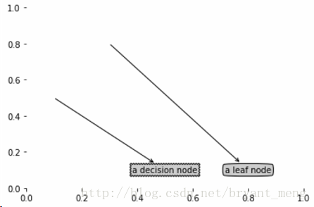
plotNode('a decision node', (0.5, 0.1), (0.1, 0.5), decisionNode)
#第一个坐标是矩形的中心点坐标,第二个是剪头起始点的坐标
plotNode('a leaf node', (0.8, 0.1), (0.3, 0.8), leafNode)
plt.show()
# 把树的信息提前存储好了,以免每次测试代码的时候,
def retrieveTree(i):
listOfTrees =[{'no surfacing': {0: 'no', 1: {'flippers': {0: 'no', 1: 'yes'}}}},
{'no surfacing': {0: 'no', 1: {'flippers': {0: {'head': {0: 'no', 1: 'yes'}}, 1: 'no'}}}}
]
return listOfTrees[i]
#createPlot(thisTree)2.1 Matplotlib注解
import matplotlib.pyplot as plt
import treePlotter
treePlotter.createPlot()
结果为
2.2 构造注解树
myDat,labels = trees.createDataSet()
myTree = trees.createTree(myDat,labels)
print (myTree)
print ('number of leaves:',treePlotter.getNumLeafs(myTree))
print ('depth of the tree:',treePlotter.getTreeDepth(myTree))
结果为
{'no surfacing': {0: 'no', 1: {'flippers': {0: 'no', 1: 'yes'}}}}
number of leaves: 3
depth of the tree: 2
画出树
treePlotter.createPlot1(myTree)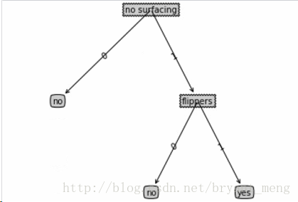
3 测试
加载数据集
fr = open('lenses.txt')
lenses = [inst.strip().split('\t') for inst in fr.readlines()]
lensesLabels = ['age', 'prescript', 'astigmatic', 'tearRate']
lensesTree = trees.createTree(lenses,lensesLabels)
print (lensesTree)
treePlotter.createPlot1(lensesTree)
结果为
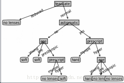
数据集如下
前四列是特征,最后一列是标签
四个特征分别是age(3种属性)、prescript(2)、astigmatic(2)、tearRate(2)
young   myope   no  reduced no lenses
young   myope   no  normal  soft
young   myope   yes reduced no lenses
young   myope   yes normal  hard
young   hyper   no  reduced no lenses
young   hyper   no  normal  soft
young   hyper   yes reduced no lenses
young   hyper   yes normal  hard
pre myope   no  reduced no lenses
pre myope   no  normal  soft
pre myope   yes reduced no lenses
pre myope   yes normal  hard
pre hyper   no  reduced no lenses
pre hyper   no  normal  soft
pre hyper   yes reduced no lenses
pre hyper   yes normal  no lenses
presbyopic  myope   no  reduced no lenses
presbyopic  myope   no  normal  no lenses
presbyopic  myope   yes reduced no lenses
presbyopic  myope   yes normal  hard
presbyopic  hyper   no  reduced no lenses
presbyopic  hyper   no  normal  soft
presbyopic  hyper   yes reduced no lenses
presbyopic  hyper   yes normal  no lenses