OpenCV(Python3)_11(图像的阀值)

目标

在本教程中，您将学习简单阈值，自适应阈值，OSTU阈值等。
您将学习这些功能：cv.threshold，cv.adaptiveThreshold等。

简单的阈值

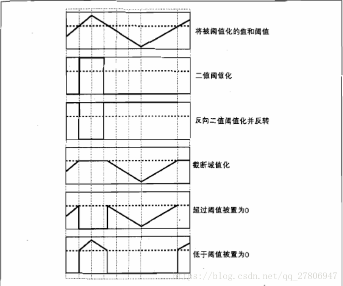
这里，问题很简单。如果像素值大于阈值，则会赋予一个新值（可能为白色），否则会分配另一个值（可能为黑色）。使用的函数是cv.threshold。这个函数的第一个参数是原图像，原图像应该是灰度图像。第二个参数是用于分类像素值的阈值。第三个参数是maxVal，它表示在像素值大于（有时小于）阈值时，应该要赋予的值。OpenCV提供不同风格的阈值，并由函数的第四个参数决定。不同的类型是：

文档清楚地解释了每种类型的含义。请查看文档。

获得两个输出。第一个是后面将解释的retval。第二个输出是我们的阈值图像。

程序：

import cv2 as cv
import numpy as np
from matplotlib import pyplot as plt
img = cv.imread('lena.jpg',0)
ret,thresh1 = cv.threshold(img,127,255,cv.THRESH_BINARY)
ret,thresh2 = cv.threshold(img,127,255,cv.THRESH_BINARY_INV)
ret,thresh3 = cv.threshold(img,127,255,cv.THRESH_TRUNC)
ret,thresh4 = cv.threshold(img,127,255,cv.THRESH_TOZERO)
ret,thresh5 = cv.threshold(img,127,255,cv.THRESH_TOZERO_INV)
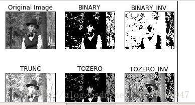
titles = ['Original Image','BINARY','BINARY_INV','TRUNC','TOZERO','TOZERO_INV']
images = [img, thresh1, thresh2, thresh3, thresh4, thresh5]
for i in range(6):

plt.subplot(2,3,i+1),plt.imshow(images[i],'gray')

plt.title(titles[i])
plt.xticks([]),plt.yticks([])

plt.show()

注意: 要绘制多个图像，我们使用了plt.subplot（）函数。请检查Matplotlib文档的更多细节。

结果如下：

自适应阈值

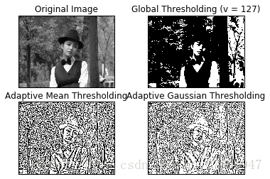
在前一节中，我们使用了一个全局值作为阈值。但是，这种方法并不适用于所有的情况，特别是图像的不同区域部分具有不同亮度时。在这种情况下，我们需要采用自适应阈值处理。该算法会根据图像上不同的小区域，从而计算出不同的阈值。因此，我们针对同一图像的不同区域会采用不同的阈值，从而使得我们能在亮度不同的情况下，得到更好的结果。

它有三个输入参数和一个输出参数。

Adaptive Method - 决定如何计算阈值。

cv.ADAPTIVE_THRESH_MEAN_C：阈值是相邻区域的平均值。
cv.ADAPTIVE_THRESH_GAUSSIAN_C：阈值是相邻区域的加权和，权重是一个高斯窗口。

Block Size - 决定邻域的大小。

C - 它只是一个从平均值或加权平均值中减去的常数。

下面的一段代码比较了全局阈值和自适应阈值对于不同照度的图像：

程序：

import cv2 as cv
import numpy as np
from matplotlib import pyplot as plt
img = cv.imread('lena.jpg',0)
img = cv.medianBlur(img,5)

ret,th1 = cv.threshold(img,127,255,cv.THRESH_BINARY)

#图像，maxval,方法，阀值类型，blocksize,C

th2 = cv.adaptiveThreshold(img,255,cv.ADAPTIVE_THRESH_MEAN_C, cv.THRESH_BINARY,11,2)
th3 = cv.adaptiveThreshold(img,255,cv.ADAPTIVE_THRESH_GAUSSIAN_C,cv.THRESH_BINARY,11,2)
titles = ['Original Image', 'Global Thresholding (v = 127)','Adaptive Mean Thresholding', 'Adaptive Gaussian Thresholding']
images = [img, th1, th2, th3]
for i in range(4):
    plt.subplot(2,2,i+1),plt.imshow(images[i],'gray')
    plt.title(titles[i])
    plt.xticks([]),plt.yticks([])
plt.show()

结果：

OSTU的二值化

在第一部分中我们提到过 retVal，当我们使用 Otsu 二值化时会用到它。那么它到底是什么呢？

在使用全局阈值时，我们就是随便给了一个数来做阈值，那我们怎么知道我们选取的这个数的好坏呢？答案就是不停的尝试。如果是一副双峰图像（简单来说双峰图像是指图像直方图中存在两个峰）呢？我们岂不是应该在两个峰之间的峰谷选一个值作为阈值？这就是 Otsu 二值化要做的。简单来说就是对一副双峰图像自动根据其直方图计算出一个阈值。（对于非双峰图像，这种方法得到的结果可能会不理想）。

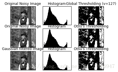
这里用到到的函数还是 cv2.threshold()，但是需要多传入一个参数（flag）：cv2.THRESH_OTSU。这时要把阈值设为 0。然后算法会找到最优阈值，这个最优阈值就是返回值 retVal。如果不使用 Otsu 二值化，返回的retVal 值与设定的阈值相等。下面的例子中，输入图像是一副带有噪声的图像。第一种方法，我们设127 为全局阈值。第二种方法，我们直接使用 Otsu 二值化。第三种方法，我们首先使用一个 5x5 的高斯核除去噪音，然后再使用 Otsu 二值化。看看噪音去除对结果的影响有多大吧。

程序：

import cv2 as cv
import numpy as np
from matplotlib import pyplot as plt
img = cv.imread('lena.jpg',0)
# global thresholding
ret1,th1 = cv.threshold(img,127,255,cv.THRESH_BINARY)
# Otsu's thresholding
ret2,th2 = cv.threshold(img,0,255,cv.THRESH_BINARY+cv.THRESH_OTSU)
# Otsu's thresholding after Gaussian filtering
blur = cv.GaussianBlur(img,(5,5),0)
ret3,th3 = cv.threshold(blur,0,255,cv.THRESH_BINARY+cv.THRESH_OTSU)
# plot all the images and their histograms
images = [img, 0, th1,
          img, 0, th2,
          blur, 0, th3]
titles = ['Original Noisy Image','Histogram','Global Thresholding (v=127)',
          'Original Noisy Image','Histogram',"Otsu's Thresholding",
          'Gaussian filtered Image','Histogram',"Otsu's Thresholding"]
for i in range(3):
    plt.subplot(3,3,i*3+1),plt.imshow(images[i*3],'gray')
    plt.title(titles[i*3]), plt.xticks([]), plt.yticks([])
    plt.subplot(3,3,i*3+2),plt.hist(images[i*3].ravel(),256)
    plt.title(titles[i*3+1]), plt.xticks([]), plt.yticks([])
    plt.subplot(3,3,i*3+3),plt.imshow(images[i*3+2],'gray')
    plt.title(titles[i*3+2]), plt.xticks([]), plt.yticks([])

plt.show()

#plt.hist(images[i*3].ravel(),256) 是绘制图像直方图，ravel是将图像的多维数组降维，变成一维数组，256是将横轴分为256组。

结果如下：

OSTU算法原理：

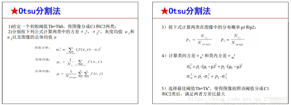
我觉得这个解释更好。

程序：

import cv2 as cv
import numpy as np
from matplotlib import pyplot as plt

img = cv.imread('lena.jpg',0)
blur = cv.GaussianBlur(img,(5,5),0)
# find normalized_histogram, and its cumulative distribution function
#image ,通道，MASK，分为多少份，像素范围
hist = cv.calcHist([blur],[0],None,[256],[0,256])
#归一化
hist_norm = hist.ravel()/hist.max()
Q = hist_norm.cumsum()
bins = np.arange(256)
fn_min = np.inf
thresh = -1
for i in range(1,256):
    p1,p2 = np.hsplit(hist_norm,[i]) # probabilities
    q1,q2 = Q[i],Q[255]-Q[i] # cum sum of classes
    b1,b2 = np.hsplit(bins,[i]) # weights
    # finding means and variances
    m1,m2 = np.sum(p1*b1)/q1, np.sum(p2*b2)/q2
    v1,v2 = np.sum(((b1-m1)**2)*p1)/q1,np.sum(((b2-m2)**2)*p2)/q2
    # calculates the minimization function
    fn = v1*q1 + v2*q2
    if fn < fn_min:
        fn_min = fn
        thresh = i
# find otsu's threshold value with OpenCV function
ret, otsu = cv.threshold(blur,0,255,cv.THRESH_BINARY+cv.THRESH_OTSU)
print( "{} {}".format(thresh,ret) )

结果：

测试结果还是很相近的！